Fixed error
Source Link
Michael E2
  • 244.8k
  • 18
  • 351
  • 774

If you solve for the second derivatives, you won't have to use "EquationSimplification" -> "Residual" and things will work ok.

Solving for the second derivatives be faster if you start with exact coefficients. Also, if you clear l, solve for the derivatives, and then substitute a value for l, Solve won't choke on the algebra. The long time it takes is probably why NDSolve advises the use of the option:

NDSolve::ntdv: Cannot solve to find an explicit formula for the derivatives. Consider using the option Method->{"EquationSimplification"->"Residual"}. >>

l(*l = 0.6 (1 + 0.00 I) // Rationalize;Rationalize;*)  (* old solution *)
Clear[l];
g = 9.8 // Rationalize;
x0 = 0.01 // Rationalize;
(*... rest of OP's code...*)

(* This replaces eq[] in NDSolve; saves the result for ease of reuse *)
Clear[neweq];
neweq[n_, ω0_] := neweq[n, ω0] = 
  Equal @@@ First@ Simplify@
     Solve[eq[n] /. ω -> ω0, Table[Subscript[x, i]''[t], {i, n}]] 

(* Here is where we substitute the value for l *)
Clear[SOL];
SOL[n_] := NDSolve[{neweq[n, 1] /. l -> 0.6 (1 + 0.01 I), ic[n]},
  Table[Subscript[x, i][t], {i, n}], {t, 0, 100}]

mysol = First@SOL[4]

TheSince the solutions are complex, one has to decide what to plot. I chose the magnitude. The plots nearly overlap, so I offset them:

Plot[
 0.01 Range[n] + Table[Subscript[xTable[Abs@ Subscript[x, i][t], {i, n}] /. mysol // Evaluate,
 {t, 0, 100}]

Mathematica graphicsMathematica graphics

If you solve for the second derivatives, you won't have to use "EquationSimplification" -> "Residual" and things will work ok.

Solving for the second derivatives be faster if you start with exact coefficients. The long time it takes is probably why NDSolve advises the use of the option:

NDSolve::ntdv: Cannot solve to find an explicit formula for the derivatives. Consider using the option Method->{"EquationSimplification"->"Residual"}. >>

l = 0.6 (1 + 0.00 I) // Rationalize;
g = 9.8 // Rationalize;
x0 = 0.01 // Rationalize;
(*... rest of OP's code...*)

(* This replaces eq[] in NDSolve; saves the result for ease of reuse *)
Clear[neweq];
neweq[n_, ω0_] := neweq[n, ω0] = 
  Equal @@@ First@ Simplify@
     Solve[eq[n] /. ω -> ω0, Table[Subscript[x, i]''[t], {i, n}]]

Clear[SOL];
SOL[n_] := NDSolve[{neweq[n, 1], ic[n]}, Table[Subscript[x, i][t], {i, n}], {t, 0, 100}]

mysol = First@SOL[4]

The plots nearly overlap, so I offset them:

Plot[
 0.01 Range[n] + Table[Subscript[x, i][t], {i, n}] /. mysol // Evaluate,
 {t, 0, 100}]
Mathematica graphics

If you solve for the second derivatives, you won't have to use "EquationSimplification" -> "Residual" and things will work ok.

Solving for the second derivatives be faster if you start with exact coefficients. Also, if you clear l, solve for the derivatives, and then substitute a value for l, Solve won't choke on the algebra. The long time it takes is probably why NDSolve advises the use of the option:

NDSolve::ntdv: Cannot solve to find an explicit formula for the derivatives. Consider using the option Method->{"EquationSimplification"->"Residual"}. >>

(*l = 0.6 (1 + 0.00 I) // Rationalize;*)  (* old solution *)
Clear[l];
g = 9.8 // Rationalize;
x0 = 0.01 // Rationalize;
(*... rest of OP's code...*)

(* This replaces eq[] in NDSolve; saves the result for ease of reuse *)
Clear[neweq];
neweq[n_, ω0_] := neweq[n, ω0] = 
  Equal @@@ First@ Simplify@
     Solve[eq[n] /. ω -> ω0, Table[Subscript[x, i]''[t], {i, n}]] 

(* Here is where we substitute the value for l *)
Clear[SOL];
SOL[n_] := NDSolve[{neweq[n, 1] /. l -> 0.6 (1 + 0.01 I), ic[n]},
  Table[Subscript[x, i][t], {i, n}], {t, 0, 100}]

mysol = First@SOL[4]

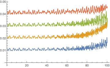
Since the solutions are complex, one has to decide what to plot. I chose the magnitude. The plots nearly overlap, so I offset them:

Plot[
 0.01 Range[n] + Table[Abs@ Subscript[x, i][t], {i, n}] /. mysol // Evaluate,
 {t, 0, 100}]

Mathematica graphics

Source Link
Michael E2
  • 244.8k
  • 18
  • 351
  • 774

If you solve for the second derivatives, you won't have to use "EquationSimplification" -> "Residual" and things will work ok.

Solving for the second derivatives be faster if you start with exact coefficients. The long time it takes is probably why NDSolve advises the use of the option:

NDSolve::ntdv: Cannot solve to find an explicit formula for the derivatives. Consider using the option Method->{"EquationSimplification"->"Residual"}. >>

l = 0.6 (1 + 0.00 I) // Rationalize;
g = 9.8 // Rationalize;
x0 = 0.01 // Rationalize;
(*... rest of OP's code...*)

(* This replaces eq[] in NDSolve; saves the result for ease of reuse *)
Clear[neweq];
neweq[n_, ω0_] := neweq[n, ω0] = 
  Equal @@@ First@ Simplify@
     Solve[eq[n] /. ω -> ω0, Table[Subscript[x, i]''[t], {i, n}]]

Clear[SOL];
SOL[n_] := NDSolve[{neweq[n, 1], ic[n]}, Table[Subscript[x, i][t], {i, n}], {t, 0, 100}]

mysol = First@SOL[4]

The plots nearly overlap, so I offset them:

Plot[
 0.01 Range[n] + Table[Subscript[x, i][t], {i, n}] /. mysol // Evaluate,
 {t, 0, 100}]

Mathematica graphics