fixed minor typo
Source Link
bbgodfrey
  • 62.1k
  • 18
  • 92
  • 160

The plot in the question must have been obtained with stepsizestepSize = 15, not stepsizestepSize = 2. Using the latter value gives a smooth plot,

enter image description here

The computation takes about 78 sec on my PC. To address the specific issue in the question, the run time can be reduced by two orders of magnitude using

Block[{stepSize = 2, end = TMax, tt, rd}, 
    tSolpbc = Table[uSolpbc[tt, 0], {tt, 0, end, stepSize}]; 
    rd = ParallelTable[
        UnitStep[0.01 - Norm[tSolpbc[[nt]] - tSolpbc[[nτ]], 2]], 
        {nt, end/stepSize}, {nτ, end/stepSize}]; MatrixPlot[rd]]

which produces the same plot. Evidently, most of the run time used in the original computation was consumed by computing uSolpbc (end/stepSize)^2 times. The revised computation computes it only end/stepSize times.

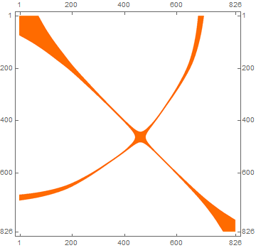
The plot in the question must have been obtained with stepsize = 15, not stepsize = 2. Using the latter value gives a smooth plot,

enter image description here

The computation takes about 78 sec on my PC. To address the specific issue in the question, the run time can be reduced by two orders of magnitude using

Block[{stepSize = 2, end = TMax, tt, rd}, 
    tSolpbc = Table[uSolpbc[tt, 0], {tt, 0, end, stepSize}]; 
    rd = ParallelTable[
        UnitStep[0.01 - Norm[tSolpbc[[nt]] - tSolpbc[[nτ]], 2]], 
        {nt, end/stepSize}, {nτ, end/stepSize}]; MatrixPlot[rd]]

which produces the same plot. Evidently, most of the run time used in the original computation was consumed by computing uSolpbc (end/stepSize)^2 times. The revised computation computes it only end/stepSize times.

The plot in the question must have been obtained with stepSize = 15, not stepSize = 2. Using the latter value gives a smooth plot,

enter image description here

The computation takes about 78 sec on my PC. To address the specific issue in the question, the run time can be reduced by two orders of magnitude using

Block[{stepSize = 2, end = TMax, tt, rd}, 
    tSolpbc = Table[uSolpbc[tt, 0], {tt, 0, end, stepSize}]; 
    rd = ParallelTable[
        UnitStep[0.01 - Norm[tSolpbc[[nt]] - tSolpbc[[nτ]], 2]], 
        {nt, end/stepSize}, {nτ, end/stepSize}]; MatrixPlot[rd]]

which produces the same plot. Evidently, most of the run time used in the original computation was consumed by computing uSolpbc (end/stepSize)^2 times. The revised computation computes it only end/stepSize times.

added last two sentences.
Source Link
bbgodfrey
  • 62.1k
  • 18
  • 92
  • 160

The plot in the question must have been obtained with stepsize = 15, not stepsize = 2. Using the latter value gives a smooth plot,

enter image description here

The computation takes about 78 sec on my PC. To address the specific issue in the question, the run time can be reduced by two orders of magnitude using,

Block[{stepSize = 2, end = TMax, tt, ττ, rd}, 
    tSolpbc = Table[uSolpbc[tt, 0], {tt, 0, end, stepSize}]; 
    rd = ParallelTable[
        UnitStep[0.01 - Norm[tSolpbc[[nt]] - tSolpbc[[nτ]], 2]], 
        {nt, end/stepSize}, {nτ, end/stepSize}]; MatrixPlot[rd]]

which produces the same plot. Evidently, most of the run time used in the original computation was consumed by computing uSolpbc (end/stepSize)^2 times. The revised computation computes it only end/stepSize times.

The plot in the question must have been obtained with stepsize = 15, not stepsize = 2. Using the latter value gives a smooth plot,

enter image description here

The computation takes about 78 sec on my PC. To address the specific issue in the question, the run time can be reduced by two orders of magnitude using,

Block[{stepSize = 2, end = TMax, tt, ττ, rd}, 
    tSolpbc = Table[uSolpbc[tt, 0], {tt, 0, end, stepSize}]; 
    rd = ParallelTable[
        UnitStep[0.01 - Norm[tSolpbc[[nt]] - tSolpbc[[nτ]], 2]], 
        {nt, end/stepSize}, {nτ, end/stepSize}]; MatrixPlot[rd]]

which produces the same plot.

The plot in the question must have been obtained with stepsize = 15, not stepsize = 2. Using the latter value gives a smooth plot,

enter image description here

The computation takes about 78 sec on my PC. To address the specific issue in the question, the run time can be reduced by two orders of magnitude using

Block[{stepSize = 2, end = TMax, tt, rd}, 
    tSolpbc = Table[uSolpbc[tt, 0], {tt, 0, end, stepSize}]; 
    rd = ParallelTable[
        UnitStep[0.01 - Norm[tSolpbc[[nt]] - tSolpbc[[nτ]], 2]], 
        {nt, end/stepSize}, {nτ, end/stepSize}]; MatrixPlot[rd]]

which produces the same plot. Evidently, most of the run time used in the original computation was consumed by computing uSolpbc (end/stepSize)^2 times. The revised computation computes it only end/stepSize times.

Source Link
bbgodfrey
  • 62.1k
  • 18
  • 92
  • 160

The plot in the question must have been obtained with stepsize = 15, not stepsize = 2. Using the latter value gives a smooth plot,

enter image description here

The computation takes about 78 sec on my PC. To address the specific issue in the question, the run time can be reduced by two orders of magnitude using,

Block[{stepSize = 2, end = TMax, tt, ττ, rd}, 
    tSolpbc = Table[uSolpbc[tt, 0], {tt, 0, end, stepSize}]; 
    rd = ParallelTable[
        UnitStep[0.01 - Norm[tSolpbc[[nt]] - tSolpbc[[nτ]], 2]], 
        {nt, end/stepSize}, {nτ, end/stepSize}]; MatrixPlot[rd]]

which produces the same plot.