added 6 characters in body
Source Link
m_goldberg
  • 108.1k
  • 16
  • 104
  • 259

This is not a answer, but an extended comment.

Here is your code cleaned up (I reduce the number of iterations from 10 to 3 to save space).

β1 = 0.;
β2 = N[Pi];
β3 = 0.;
a[t_] = 
  {{E^(I*β1 + I*β3)*Cos[β2*t], E^(I*β1 - I*β3)*Sin[β2*t]}, 
   {(-E^((-I)*β1 + I*β3))*Sin[β2*t], E^((-I)*β1 - I*β3)*Cos[β2*t]}} // Chop

{{1. Cos[3.14159 t], 1. Sin[3.14159 t]}, {-1. Sin[3.14159 t], 1. Cos[3.14159 t]}}

Note that there are no complex values.

tu = Module[{t = 0.},Table[t += 1. + TimeUsed[]; Print[a[t]]; i, 3]]

output

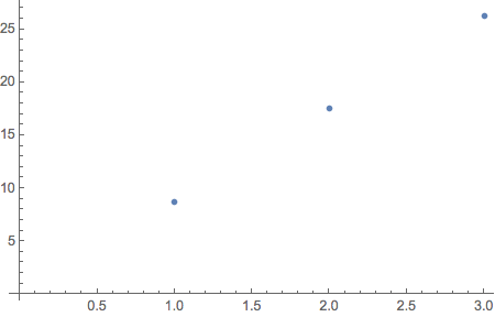
{8.7486, 17.4973, 26.2461}

ListPlot[tu]

plot

The printed values of the matix a[t] are all real-valued, but are not captured by your algorithm. They could had by making a simple modification.

Module[{t = 0.}, Table[t += 1. + TimeUsed[]; a[t], 3]]

{{{-0.74568, 0.666305}, {-0.666305, -0.74568}}, {{0.112157, -0.99369}, {0.99369, 0.112157}}, {{0.578378, 0.815769}, {-0.815769, 0.578378}}}

However, I can not understand from your question how you expect to make a plot of a list of 2 x 2 matrices. Can you make your intent clearer?

This is not a answer, but an extended comment.

Here is your code cleaned up (I reduce the number of iterations from 10 to 3 to save space).

β1 = 0.;
β2 = N[Pi];
β3 = 0.;
a[t_] = 
  {{E^(I*β1 + I*β3)*Cos[β2*t], E^(I*β1 - I*β3)*Sin[β2*t]}, 
   {(-E^((-I)*β1 + I*β3))*Sin[β2*t], E^((-I)*β1 - I*β3)*Cos[β2*t]}} // Chop

{{1. Cos[3.14159 t], 1. Sin[3.14159 t]}, {-1. Sin[3.14159 t], 1. Cos[3.14159 t]}}

Note that are no complex values.

tu = Module[{t = 0.},Table[t += 1. + TimeUsed[]; Print[a[t]]; i, 3]]

output

{8.7486, 17.4973, 26.2461}

ListPlot[tu]

plot

The printed values of the matix a[t] are all real-valued, but are not captured by your algorithm. They could had by making a simple modification.

Module[{t = 0.}, Table[t += 1. + TimeUsed[]; a[t], 3]]

{{{-0.74568, 0.666305}, {-0.666305, -0.74568}}, {{0.112157, -0.99369}, {0.99369, 0.112157}}, {{0.578378, 0.815769}, {-0.815769, 0.578378}}}

However, I can not understand from your question how you expect to make a plot of a list of 2 x 2 matrices. Can you make your intent clearer?
This is not a answer, but an extended comment.

Here is your code cleaned up (I reduce the number of iterations from 10 to 3 to save space).

β1 = 0.;
β2 = N[Pi];
β3 = 0.;
a[t_] = 
  {{E^(I*β1 + I*β3)*Cos[β2*t], E^(I*β1 - I*β3)*Sin[β2*t]}, 
   {(-E^((-I)*β1 + I*β3))*Sin[β2*t], E^((-I)*β1 - I*β3)*Cos[β2*t]}} // Chop

{{1. Cos[3.14159 t], 1. Sin[3.14159 t]}, {-1. Sin[3.14159 t], 1. Cos[3.14159 t]}}

Note that there are no complex values.

tu = Module[{t = 0.},Table[t += 1. + TimeUsed[]; Print[a[t]]; i, 3]]

output

{8.7486, 17.4973, 26.2461}

ListPlot[tu]

plot

The printed values of the matix a[t] are all real-valued, but are not captured by your algorithm. They could had by making a simple modification.

Module[{t = 0.}, Table[t += 1. + TimeUsed[]; a[t], 3]]

{{{-0.74568, 0.666305}, {-0.666305, -0.74568}}, {{0.112157, -0.99369}, {0.99369, 0.112157}}, {{0.578378, 0.815769}, {-0.815769, 0.578378}}}

However, I can not understand from your question how you expect to make a plot of a list of 2 x 2 matrices. Can you make your intent clearer?

added 1 character in body
Source Link
m_goldberg
  • 108.1k
  • 16
  • 104
  • 259

This is not a answer, but an extended comment.

Here is your code cleaned up (I reduce the number of iterations from 10 to 3 to save space).

β1 = 0.;
β2 = N[Pi];
β3 = 0.;
a[t_] = 
  {{E^(I*β1 + I*β3)*Cos[β2*t], E^(I*β1 - I*β3)*Sin[β2*t]}, 
   {(-E^((-I)*β1 + I*β3))*Sin[β2*t], E^((-I)*β1 - I*β3)*Cos[β2*t]}} // Chop

{{1. Cos[3.14159 t], 1. Sin[3.14159 t]}, {-1. Sin[3.14159 t], 1. Cos[3.14159 t]}}

Note that are no complex values.

tu = Module[{t = 0.},Table[t += 1. + TimeUsed[]; Print[a[t]]; i, 3]]

output

{8.7486, 17.4973, 26.2461}

ListPlot[tu]

plot

The printed values of the matix a[t] are all real-valued, but are not captured by your algorithm. They could had by making a simple modification.

Module[{t = 0.}, Table[t += 1. + TimeUsed[]; a[t], 3]]

{{{-0.74568, 0.666305}, {-0.666305, -0.74568}}, {{0.112157, -0.99369}, {0.99369, 0.112157}}, {{0.578378, 0.815769}, {-0.815769, 0.578378}}}

However, I can not understand from your question how you expect to make a plot of a list of 2 x 2 matrices. Can you make your intent clearer?

This is not a answer, but an extended comment.

Here is your code cleaned up (I reduce the number of iterations from 10 to 3 to save space.

β1 = 0.;
β2 = N[Pi];
β3 = 0.;
a[t_] = 
  {{E^(I*β1 + I*β3)*Cos[β2*t], E^(I*β1 - I*β3)*Sin[β2*t]}, 
   {(-E^((-I)*β1 + I*β3))*Sin[β2*t], E^((-I)*β1 - I*β3)*Cos[β2*t]}} // Chop

{{1. Cos[3.14159 t], 1. Sin[3.14159 t]}, {-1. Sin[3.14159 t], 1. Cos[3.14159 t]}}

Note that are no complex values.

tu = Module[{t = 0.},Table[t += 1. + TimeUsed[]; Print[a[t]]; i, 3]]

output

{8.7486, 17.4973, 26.2461}

ListPlot[tu]

plot

The printed values of the matix a[t] are all real-valued, but are not captured by your algorithm. They could had by making a simple modification.

Module[{t = 0.}, Table[t += 1. + TimeUsed[]; a[t], 3]]

{{{-0.74568, 0.666305}, {-0.666305, -0.74568}}, {{0.112157, -0.99369}, {0.99369, 0.112157}}, {{0.578378, 0.815769}, {-0.815769, 0.578378}}}

However, I can not understand from your question how you expect to make a plot of a list of 2 x 2 matrices. Can you make your intent clearer?

This is not a answer, but an extended comment.

Here is your code cleaned up (I reduce the number of iterations from 10 to 3 to save space).

β1 = 0.;
β2 = N[Pi];
β3 = 0.;
a[t_] = 
  {{E^(I*β1 + I*β3)*Cos[β2*t], E^(I*β1 - I*β3)*Sin[β2*t]}, 
   {(-E^((-I)*β1 + I*β3))*Sin[β2*t], E^((-I)*β1 - I*β3)*Cos[β2*t]}} // Chop

{{1. Cos[3.14159 t], 1. Sin[3.14159 t]}, {-1. Sin[3.14159 t], 1. Cos[3.14159 t]}}

Note that are no complex values.

tu = Module[{t = 0.},Table[t += 1. + TimeUsed[]; Print[a[t]]; i, 3]]

output

{8.7486, 17.4973, 26.2461}

ListPlot[tu]

plot

The printed values of the matix a[t] are all real-valued, but are not captured by your algorithm. They could had by making a simple modification.

Module[{t = 0.}, Table[t += 1. + TimeUsed[]; a[t], 3]]

{{{-0.74568, 0.666305}, {-0.666305, -0.74568}}, {{0.112157, -0.99369}, {0.99369, 0.112157}}, {{0.578378, 0.815769}, {-0.815769, 0.578378}}}

However, I can not understand from your question how you expect to make a plot of a list of 2 x 2 matrices. Can you make your intent clearer?

Source Link
m_goldberg
  • 108.1k
  • 16
  • 104
  • 259

This is not a answer, but an extended comment.

Here is your code cleaned up (I reduce the number of iterations from 10 to 3 to save space.

β1 = 0.;
β2 = N[Pi];
β3 = 0.;
a[t_] = 
  {{E^(I*β1 + I*β3)*Cos[β2*t], E^(I*β1 - I*β3)*Sin[β2*t]}, 
   {(-E^((-I)*β1 + I*β3))*Sin[β2*t], E^((-I)*β1 - I*β3)*Cos[β2*t]}} // Chop

{{1. Cos[3.14159 t], 1. Sin[3.14159 t]}, {-1. Sin[3.14159 t], 1. Cos[3.14159 t]}}

Note that are no complex values.

tu = Module[{t = 0.},Table[t += 1. + TimeUsed[]; Print[a[t]]; i, 3]]

output

{8.7486, 17.4973, 26.2461}

ListPlot[tu]

plot

The printed values of the matix a[t] are all real-valued, but are not captured by your algorithm. They could had by making a simple modification.

Module[{t = 0.}, Table[t += 1. + TimeUsed[]; a[t], 3]]

{{{-0.74568, 0.666305}, {-0.666305, -0.74568}}, {{0.112157, -0.99369}, {0.99369, 0.112157}}, {{0.578378, 0.815769}, {-0.815769, 0.578378}}}

However, I can not understand from your question how you expect to make a plot of a list of 2 x 2 matrices. Can you make your intent clearer?