Improve the English
Source Link
Jack LaVigne
  • 14.5k
  • 2
  • 26
  • 37

Note that we use NumericQ for all of the input arguments to lhs. This is important when we plotwill be required the results are plotted.

The case is covered where delta is 0zero for a particular parameter.

Now I'll plot the results for the first set of parameters. For the large spread in the s values, 20.3 to 23.1 I had to increase the delta's had to be increased or the min and max were too close to be visible.

and indeed testing shows that it does indeed produce a smaller minimum:

Note that we use NumericQ for all of the input arguments to lhs. This is important when we plot the results.

The case is covered where delta is 0 for a particular parameter.

Now I'll plot the results for the first set of parameters. For the large spread in the s values, 20.3 to 23.1 I had to increase the delta's or the min and max were too close to be visible.

and indeed testing shows that it does indeed produce a smaller minimum:

Note that we use NumericQ for all of the input arguments to lhs. This will be required the results are plotted.

The case is covered where delta is zero for a particular parameter.

Now plot the results for the first set of parameters. For the large spread in the s values the delta's had to be increased or the min and max were too close to be visible.

and indeed testing shows that it does produce a smaller minimum:

Improved the speed and accuracy of the computation
Source Link
Jack LaVigne
  • 14.5k
  • 2
  • 26
  • 37

Numerical Derivatives and a faster version

If one were able to ascertain the polarity that a change in a parameter has on the outcome one could construct a faster version by reducing the number of permutations.

testDeriv = With[
  {
   a1 = -23.29,
   b1 = 0.88,
   c1 = 20.82
   },
  Table[
   {s, (lhs[s, a1 + 0.001, b1, c1] - lhs[s, a1, b1, c1])/0.001,
    (lhs[s, a1, b1 + 0.001, c1] - lhs[s, a1, b1, c1])/0.001,
    (lhs[s, a1, b1, c1 + 0.001] - lhs[s, a1, b1, c1])/0.001},
   {s, 20.3, 23.3, 0.5}
   ]
  ]

(* {{20.3, 0.00672811, 0.00102687, 0.0117371}, {20.8, 
  0.00194452, -0.000360691, 0.00494013}, {21.3, 
  0.000116524, -0.0000671435, 0.000553761}, {21.8, 
  7.0401*10^-8, -7.15508*10^-8, 8.08399*10^-7}, {22.3, 
  2.90222*10^-17, -4.32226*10^-17, 9.63237*10^-16}, {22.8, 
  4.69431*10^-46, -9.28372*10^-46, 5.11146*10^-44}, {23.3, 
  3.58277*10^-136, -8.85485*10^-136, 1.5721*10^-133}} *)

It appears that the derivative of lhs with respect to a and c is always positive and with respect to b may be either positive or negative.

Using that hypothesis a faster version of the lhs for intervals would be:

lhsMinus2[s_?NumericQ, a_?NumericQ, da_?NumericQ, b_?NumericQ, 
  db_?NumericQ, c_?NumericQ, dc_?NumericQ] := Module[
  {
   aList,
   bList,
   cList
   },
  aList = If[da == 0, {a}, {a - da}];
  bList = If[db == 0, {b}, {b, b - db, b + db}];
  cList = If[dc == 0, {c}, {c - dc}];
  
  Min[Map[lhs[s, Sequence @@ #] &, 
    Flatten[Outer[List, aList, bList, cList], 2]]]
  ]

and indeed testing shows that it does indeed produce a smaller minimum:

testMinus = With[
   {
    a1 = -23.29,
    da = 0.04,
    b1 = 0.88,
    db = 0.04,
    c1 = 20.82,
    dc = 0.01
    },
   Table[
    {s, lhsMinus[s, a1, da, b1, db, c1, dc], 
     lhsMinus2[s, a1, da, b1, db, c1, dc]},
    {s, 20.3, 23.3, 0.5}
    ]
   ];

Map[{#[[1]], #[[3]]/#[[2]]} &, testMinus]
(* {{20.3, 1.}, {20.8, 0.98248}, {21.3, 0.947516}, {21.8, 
  0.909672}, {22.3, 0.870701}, {22.8, 0.832196}, {23.3, 0.794958}} *)

The same is true for the positive side:

lhsPlus2[s_?NumericQ, a_?NumericQ, da_?NumericQ, b_?NumericQ, 
  db_?NumericQ, c_?NumericQ, dc_?NumericQ] := Module[
  {
   aList,
   bList,
   cList
   },
  aList = If[da == 0, {a}, {a + da}];
  bList = If[db == 0, {b}, {b, b - db, b + db}];
  cList = If[dc == 0, {c}, {c + dc}];
  
  Max[Map[lhs[s, Sequence @@ #] &, 
    Flatten[Outer[List, aList, bList, cList], 2]]]
  ]

testPlus = With[
  {
   a1 = -23.29,
   da = 0.04,
   b1 = 0.88,
   db = 0.04,
   c1 = 20.82,
   dc = 0.01
   },
  Table[
   {s, lhsPlus[s, a1, da, b1, db, c1, dc], 
    lhsPlus2[s, a1, da, b1, db, c1, dc]},
   {s, 20.3, 23.3, 0.5}
   ]
  ];

Map[{#[[1]], #[[3]]/#[[2]]} &, testPlus]
(* {{20.3, 1.}, {20.8, 1.01669}, {21.3, 1.05383}, {21.8, 
  1.09744}, {22.3, 1.14645}, {22.8, 1.19945}, {23.3, 1.25562}} *)
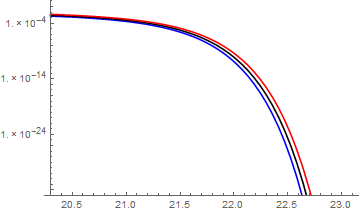
Change the plot range to be consistent with OP's question
Source Link
Jack LaVigne
  • 14.5k
  • 2
  • 26
  • 37
With[
 {
  a1 = -23.29,
  da = 0.08,
  b1 = 0.88,
  db = 0.08,
  c1 = 20.82,
  dc = 0.04
  },
 LogPlot[
  {
   lhsMinus[s, a1, da, b1, db, c1, dc],
   lhs[s, a1, b1, c1],
   lhsPlus[s, a1, da, b1, db, c1, dc]
   },
  {s, 20.3, 23.1},
  {PlotStyle -> {Blue, Black, Red}},
   PlotRange -> {10^-35, 1}
  ]
 ]

Mathematica graphicsMathematica graphics

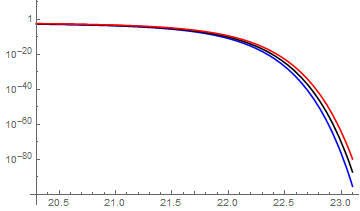
With[
 {
  a1 = -23.29,
  da = 0.08,
  b1 = 0.88,
  db = 0.08,
  c1 = 20.82,
  dc = 0.04
  },
 LogPlot[
  {
   lhsMinus[s, a1, da, b1, db, c1, dc],
   lhs[s, a1, b1, c1],
   lhsPlus[s, a1, da, b1, db, c1, dc]
   },
  {s, 20.3, 23.1},
  {PlotStyle -> {Blue, Black, Red}}
  ]
 ]

Mathematica graphics

With[
 {
  a1 = -23.29,
  da = 0.08,
  b1 = 0.88,
  db = 0.08,
  c1 = 20.82,
  dc = 0.04
  },
 LogPlot[
  {
   lhsMinus[s, a1, da, b1, db, c1, dc],
   lhs[s, a1, b1, c1],
   lhsPlus[s, a1, da, b1, db, c1, dc]
   },
  {s, 20.3, 23.1},
  {PlotStyle -> {Blue, Black, Red}},
   PlotRange -> {10^-35, 1}
  ]
 ]

Mathematica graphics

Source Link
Jack LaVigne
  • 14.5k
  • 2
  • 26
  • 37
Loading