replaced http://mathematica.stackexchange.com/ with https://mathematica.stackexchange.com/
Source Link

I recommend using Graphics primitives for this kind of application, which gives you direct (and usually easier) control of appearance. As a bonus performance is usually better as well.

For simple applications such as this, if you don't also need the plots separately, you can use Epilog in ParametricPlot to insert these primitives:

ParametricPlot[{Sin[t], Cos[t]}, {t, 0, 2 Pi}, 
  PlotStyle -> {Red, Thickness[0.01]}, 
  Epilog -> {PointSize[Large], Point@Table[{Sin[n], Cos[n]}, {n, 50}]}
]
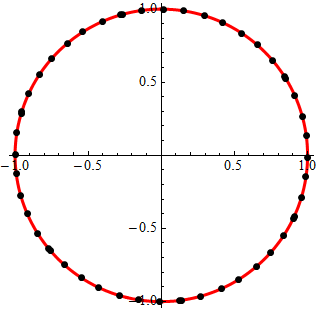
Mathematica graphics

See documentation for PointSize and AbsolutePointSize for complete control of point size.

If you need the plots separately you can do that too, like this:

p1 = ParametricPlot[{Sin[t], Cos[t]}, {t, 0, 2 Pi}, 
       PlotStyle -> {Red, Thickness[0.01]}
     ];

p2 = Graphics[
       {PointSize[Large], Point @ Table[{Sin[n], Cos[n]}, {n, 50}]},
       PlotRange -> {-1, 1}
     ];

Show[p1, p2]

In a comment J. M.J. M. reminds us that this form for p2 also works:

p2 = ListPlot[Table[{Sin[n], Cos[n]}, {n, 50}], PlotStyle -> {Black, PointSize[Large]}];

My recommendation to use graphics primitives is so that more complicated styles are within reach and so that code may be shared between Graphics and Epilog. Perhaps I am complicating things for such a simple operation and you would prefer that.

I recommend using Graphics primitives for this kind of application, which gives you direct (and usually easier) control of appearance. As a bonus performance is usually better as well.

For simple applications such as this, if you don't also need the plots separately, you can use Epilog in ParametricPlot to insert these primitives:

ParametricPlot[{Sin[t], Cos[t]}, {t, 0, 2 Pi}, 
  PlotStyle -> {Red, Thickness[0.01]}, 
  Epilog -> {PointSize[Large], Point@Table[{Sin[n], Cos[n]}, {n, 50}]}
]

Mathematica graphics

See documentation for PointSize and AbsolutePointSize for complete control of point size.

If you need the plots separately you can do that too, like this:

p1 = ParametricPlot[{Sin[t], Cos[t]}, {t, 0, 2 Pi}, 
       PlotStyle -> {Red, Thickness[0.01]}
     ];

p2 = Graphics[
       {PointSize[Large], Point @ Table[{Sin[n], Cos[n]}, {n, 50}]},
       PlotRange -> {-1, 1}
     ];

Show[p1, p2]

In a comment J. M. reminds us that this form for p2 also works:

p2 = ListPlot[Table[{Sin[n], Cos[n]}, {n, 50}], PlotStyle -> {Black, PointSize[Large]}];

My recommendation to use graphics primitives is so that more complicated styles are within reach and so that code may be shared between Graphics and Epilog. Perhaps I am complicating things for such a simple operation and you would prefer that.

added 497 characters in body
Source Link
Mr.Wizard
  • 273.1k
  • 34
  • 595
  • 1.4k

I recommend using Graphics primitives for this kind of application, which gives you direct (and usually easier) control of appearance. As a bonus performance is usually better as well.

For simple applications such as this, if you don't also need the plots separately, you can use Epilog in ParametricPlot to insert these primitives:

ParametricPlot[{Sin[t], Cos[t]}, {t, 0, 2 Pi}, 
  PlotStyle -> {Red, Thickness[0.01]}, 
  Epilog -> {PointSize[Large], Point@Table[{Sin[n], Cos[n]}, {n, 50}]}
]

Mathematica graphics

See documentation for PointSize and AbsolutePointSize for complete control of point size.

If you need the plots separately you can do that too, like this:

p1 = ParametricPlot[{Sin[t], Cos[t]}, {t, 0, 2 Pi}, 
       PlotStyle -> {Red, Thickness[0.01]}
     ];

p2 = Graphics[
       {PointSize[Large], Point @ Table[{Sin[n], Cos[n]}, {n, 50}]},
       PlotRange -> {-1, 1}
     ];

Show[p1, p2]

In a comment J. M. reminds us that this form for p2 also works:

p2 = ListPlot[Table[{Sin[n], Cos[n]}, {n, 50}], PlotStyle -> {Black, PointSize[Large]}];

My recommendation to use graphics primitives is so that more complicated styles are within reach and so that code may be shared between Graphics and Epilog. Perhaps I am complicating things for such a simple operation and you would prefer that.

I recommend using Graphics primitives for this kind of application, which gives you direct (and usually easier) control of appearance. As a bonus performance is usually better as well.

For simple applications such as this, if you don't also need the plots separately, you can use Epilog in ParametricPlot to insert these primitives:

ParametricPlot[{Sin[t], Cos[t]}, {t, 0, 2 Pi}, 
  PlotStyle -> {Red, Thickness[0.01]}, 
  Epilog -> {PointSize[Large], Point@Table[{Sin[n], Cos[n]}, {n, 50}]}
]

Mathematica graphics

See documentation for PointSize and AbsolutePointSize for complete control of point size.

If you need the plots separately you can do that too, like this:

p1 = ParametricPlot[{Sin[t], Cos[t]}, {t, 0, 2 Pi}, 
       PlotStyle -> {Red, Thickness[0.01]}
     ];

p2 = Graphics[
       {PointSize[Large], Point @ Table[{Sin[n], Cos[n]}, {n, 50}]},
       PlotRange -> {-1, 1}
     ];

Show[p1, p2]

In a comment J. M. reminds us that this form for p2 also works:

p2 = ListPlot[Table[{Sin[n], Cos[n]}, {n, 50}], PlotStyle -> {Black, PointSize[Large]}];

My recommendation to use graphics primitives is so that more complicated styles are within reach and so that code may be shared between Graphics and Epilog. Perhaps I am complicating things for such a simple operation and you would prefer that.

added 32 characters in body
Source Link
Mr.Wizard
  • 273.1k
  • 34
  • 595
  • 1.4k

I recommend using Graphics primitives for this kind of application, which gives you direct (and usually easier) control of appearance. As a bonus performance is usually better as well.

For simple applications such as this, if you don't also need the plots separately, you can use Epilog in ParametricPlot to insert these primitives:

p1 = ParametricPlot[{Sin[t], Cos[t]}, {t, 0, 2 Pi}, 
       PlotStyle -> {Red, Thickness[0.01]}
     ];

p2 =, Graphics[
     Epilog -> {PointSize[Large], Point @ Table[Point@Table[{Sin[n], Cos[n]}, {n, 50}]},
       PlotRange -> {-1, 1}
     ];

Show[p1, p2]]

Mathematica graphics

For simple applications such as this, ifSee documentation for PointSize and AbsolutePointSize for complete control of point size.

If you don't also need the plots separately, you can use Epilog in ParametricPlotdo that too, like this:

p1 = ParametricPlot[{Sin[t], Cos[t]}, {t, 0, 2 Pi}, 
       PlotStyle -> {Red, Thickness[0.01]},
     ];

p2 = EpilogGraphics[
 ->      {PointSize[Large], Point@Table[Point @ Table[{Sin[n], Cos[n]}, {n, 50}]},
]       PlotRange -> {-1, 1}
     ];

Show[p1, p2]

Mathematica graphics

I recommend using Graphics primitives for this kind of application, which gives you direct (and usually easier) control of appearance. As a bonus performance is usually better as well.

p1 = ParametricPlot[{Sin[t], Cos[t]}, {t, 0, 2 Pi}, 
       PlotStyle -> {Red, Thickness[0.01]}
     ];

p2 = Graphics[
       {PointSize[Large], Point @ Table[{Sin[n], Cos[n]}, {n, 50}]},
       PlotRange -> {-1, 1}
     ];

Show[p1, p2]

Mathematica graphics

For simple applications such as this, if you don't also need the plots separately, you can use Epilog in ParametricPlot:

ParametricPlot[{Sin[t], Cos[t]}, {t, 0, 2 Pi}, 
  PlotStyle -> {Red, Thickness[0.01]}, 
  Epilog -> {PointSize[Large], Point@Table[{Sin[n], Cos[n]}, {n, 50}]}
]

Mathematica graphics

I recommend using Graphics primitives for this kind of application, which gives you direct (and usually easier) control of appearance. As a bonus performance is usually better as well.

For simple applications such as this, if you don't also need the plots separately, you can use Epilog in ParametricPlot to insert these primitives:

ParametricPlot[{Sin[t], Cos[t]}, {t, 0, 2 Pi}, 
  PlotStyle -> {Red, Thickness[0.01]}, 
  Epilog -> {PointSize[Large], Point@Table[{Sin[n], Cos[n]}, {n, 50}]}
]

Mathematica graphics

See documentation for PointSize and AbsolutePointSize for complete control of point size.

If you need the plots separately you can do that too, like this:

p1 = ParametricPlot[{Sin[t], Cos[t]}, {t, 0, 2 Pi}, 
       PlotStyle -> {Red, Thickness[0.01]}
     ];

p2 = Graphics[
       {PointSize[Large], Point @ Table[{Sin[n], Cos[n]}, {n, 50}]},
       PlotRange -> {-1, 1}
     ];

Show[p1, p2]
Source Link
Mr.Wizard
  • 273.1k
  • 34
  • 595
  • 1.4k
Loading