added 442 characters in body
Source Link
Jason B.
  • 70.2k
  • 3
  • 144
  • 298

Working Precision giving crazy results

It was suggested to check out the results of using WorkingPrecision on the plot, so look at this mess:

LogLogPlot[
   Bλ[TEarth, λ], {λ, λL, λH},
    Frame -> True, PlotRange -> All, WorkingPrecision -> #, 
   ImageSize -> 300] & /@ {MachinePrecision/2, MachinePrecision, 
  2 MachinePrecision, $MachinePrecision}

enter image description here

The only setting that was even close to correct was the default setting. It seems the only real answer here is to wrap the function with Evaluate before plotting.

Edit Here is my original answer below, which I'm leaving in only because it shows off the version 10 function PlanckRadiationLaw, which is a little slow for sure.

@J.M. made the point of using nanometers instead of meters, and my first thought was to use atomic units instead of SI units, but you still run into the same problem when taking a LogLog plot.

The answer is to adjust your x-axis range, no reason to go all the way down to 10 nanometers, 100 nanometers is as low as most every plot goes.

Working Precision giving crazy results

It was suggested to check out the results of using WorkingPrecision on the plot, so look at this mess:

LogLogPlot[
   Bλ[TEarth, λ], {λ, λL, λH},
    Frame -> True, PlotRange -> All, WorkingPrecision -> #, 
   ImageSize -> 300] & /@ {MachinePrecision/2, MachinePrecision, 
  2 MachinePrecision, $MachinePrecision}

enter image description here

The only setting that was even close to correct was the default setting. It seems the only real answer here is to wrap the function with Evaluate before plotting.

Edit Here is my original answer below, which I'm leaving in only because it shows off the version 10 function PlanckRadiationLaw, which is a little slow for sure.

@J.M. made the point of using nanometers instead of meters, and my first thought was to use atomic units instead of SI units, but you still run into the same problem when taking a LogLog plot.

added 1359 characters in body
Source Link
Jason B.
  • 70.2k
  • 3
  • 144
  • 298

Yet, if I evaluate the function at 1e-8 I get basically zero

SoI don't know if you are takingcan call this a bug, but it seems buggy to me. Let's take a look at the log of zero? The fact isdata that ifis actually being plotted, which you go high enough in frequencycan extract using a Reap and Sow combination (low enough in wavelengththanks to @user21 for showing me this trick) then

Reap[LogLogPlot[Sow[{λ, Bλ[TEarth, λ]}]; 
     Bλ[TEarth, λ], {λ, λL, λH}, 
     Frame -> True]][[2, 1, ;; 20]] // TableForm
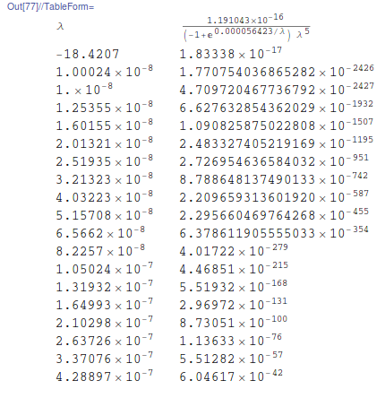
enter image description here

That would seem to be the radiation level goesbig glaring problem, right there, that point of {x,f[x]} = {-18.4207, 1.83338*10^-17}. But I'm not actually convinced, I think that is a red herring, because you get the same x value if you replace Bλ[TEarth, λ] with λ^2.

About the only thing we do learn from that table is that Mathematica doesn't seem to zero regardlesshave a problem with really small numbers.

This is apparently one of those cases where you need to use Evaluate in the units involvedargument to Plot,

GraphicsRow[{
  LogLogPlot[
   Bλ[TEarth, λ], {λ, λL, λH},
    Frame -> True],
  LogLogPlot[
   Evaluate@
    Bλ[
     TEarth, λ], {λ, λL, λH}, 
   Frame -> True]
  }, ImageSize -> 700]

enter image description here

This is a simple workaround that you can use all the time without drawback.

Edit Here is my original answer below, which I'm leaving in only because it shows off the version 10 function PlanckRadiationLaw, which is a little slow for sure.

@J.M. made the point of using nanometers instead of meters, and my first thought was to use atomic units instead of SI units, but you still run into the same problem when taking a LogLog plot.

The answer is to adjust your x-axis range, no reason to go all the way down to 10 nanometers, 100 nanometers is as low as most every plot goes.

Your code is just fine, but I thought I'd show off a version 10 function here,

LogLogPlot[{
  QuantityMagnitude[
   PlanckRadiationLaw[Quantity[5778, "Kelvins"], 
    Quantity[x, "Nanometers"]]],
  QuantityMagnitude[
   PlanckRadiationLaw[Quantity[255, "Kelvins"], 
    Quantity[x, "Nanometers"]]]}
 , {x, 10, 10^6}, 
 AxesLabel -> {Quantity[None, "Nanometers"], 
   Quantity[None, "Watts"/("Hertz"*"Meters"^2*"Steradians")]}]
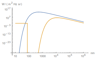
enter image description here

shows the same problem, even with proper units. But if you adjust the lowest wavelength to 100 nm, then you get this:
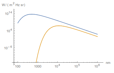
enter image description here

Yet, if I evaluate the function at 1e-8 I get basically zero

So you are taking the log of zero? The fact is that if you go high enough in frequency (low enough in wavelength) then the radiation level goes to zero regardless of the units involved.

@J.M. made the point of using nanometers instead of meters, and my first thought was to use atomic units instead of SI units, but you still run into the same problem when taking a LogLog plot.

The answer is to adjust your x-axis range, no reason to go all the way down to 10 nanometers, 100 nanometers is as low as most every plot goes.

Your code is just fine, but I thought I'd show off a version 10 function here,

LogLogPlot[{
  QuantityMagnitude[
   PlanckRadiationLaw[Quantity[5778, "Kelvins"], 
    Quantity[x, "Nanometers"]]],
  QuantityMagnitude[
   PlanckRadiationLaw[Quantity[255, "Kelvins"], 
    Quantity[x, "Nanometers"]]]}
 , {x, 10, 10^6}, 
 AxesLabel -> {Quantity[None, "Nanometers"], 
   Quantity[None, "Watts"/("Hertz"*"Meters"^2*"Steradians")]}]

enter image description here

shows the same problem, even with proper units. But if you adjust the lowest wavelength to 100 nm, then you get this:

enter image description here

I don't know if you can call this a bug, but it seems buggy to me. Let's take a look at the data that is actually being plotted, which you can extract using a Reap and Sow combination (thanks to @user21 for showing me this trick)

Reap[LogLogPlot[Sow[{λ, Bλ[TEarth, λ]}]; 
     Bλ[TEarth, λ], {λ, λL, λH}, 
     Frame -> True]][[2, 1, ;; 20]] // TableForm

enter image description here

That would seem to be the big glaring problem, right there, that point of {x,f[x]} = {-18.4207, 1.83338*10^-17}. But I'm not actually convinced, I think that is a red herring, because you get the same x value if you replace Bλ[TEarth, λ] with λ^2.

About the only thing we do learn from that table is that Mathematica doesn't seem to have a problem with really small numbers.

This is apparently one of those cases where you need to use Evaluate in the argument to Plot,

GraphicsRow[{
  LogLogPlot[
   Bλ[TEarth, λ], {λ, λL, λH},
    Frame -> True],
  LogLogPlot[
   Evaluate@
    Bλ[
     TEarth, λ], {λ, λL, λH}, 
   Frame -> True]
  }, ImageSize -> 700]

enter image description here

This is a simple workaround that you can use all the time without drawback.

Edit Here is my original answer below, which I'm leaving in only because it shows off the version 10 function PlanckRadiationLaw, which is a little slow for sure.

@J.M. made the point of using nanometers instead of meters, and my first thought was to use atomic units instead of SI units, but you still run into the same problem when taking a LogLog plot.

The answer is to adjust your x-axis range, no reason to go all the way down to 10 nanometers, 100 nanometers is as low as most every plot goes.

Your code is just fine, but I thought I'd show off a version 10 function here,

LogLogPlot[{
  QuantityMagnitude[
   PlanckRadiationLaw[Quantity[5778, "Kelvins"], 
    Quantity[x, "Nanometers"]]],
  QuantityMagnitude[
   PlanckRadiationLaw[Quantity[255, "Kelvins"], 
    Quantity[x, "Nanometers"]]]}
 , {x, 10, 10^6}, 
 AxesLabel -> {Quantity[None, "Nanometers"], 
   Quantity[None, "Watts"/("Hertz"*"Meters"^2*"Steradians")]}]

enter image description here

shows the same problem, even with proper units. But if you adjust the lowest wavelength to 100 nm, then you get this:

enter image description here

Source Link
Jason B.
  • 70.2k
  • 3
  • 144
  • 298

Yet, if I evaluate the function at 1e-8 I get basically zero

So you are taking the log of zero? The fact is that if you go high enough in frequency (low enough in wavelength) then the radiation level goes to zero regardless of the units involved.

@J.M. made the point of using nanometers instead of meters, and my first thought was to use atomic units instead of SI units, but you still run into the same problem when taking a LogLog plot.

The answer is to adjust your x-axis range, no reason to go all the way down to 10 nanometers, 100 nanometers is as low as most every plot goes.

Your code is just fine, but I thought I'd show off a version 10 function here,

LogLogPlot[{
  QuantityMagnitude[
   PlanckRadiationLaw[Quantity[5778, "Kelvins"], 
    Quantity[x, "Nanometers"]]],
  QuantityMagnitude[
   PlanckRadiationLaw[Quantity[255, "Kelvins"], 
    Quantity[x, "Nanometers"]]]}
 , {x, 10, 10^6}, 
 AxesLabel -> {Quantity[None, "Nanometers"], 
   Quantity[None, "Watts"/("Hertz"*"Meters"^2*"Steradians")]}]

enter image description here

shows the same problem, even with proper units. But if you adjust the lowest wavelength to 100 nm, then you get this:

enter image description here