replaced http://mathematica.stackexchange.com/ with https://mathematica.stackexchange.com/
Source Link

I have normally two equations system which I reduce to one equation and make its graphic. I could make the graph of the reduced equation but I can not find the appropriate command to find its root. Here is the code I use (from this answerfrom this answer) ;

u[c_] := (c^(1 - σ) - 1)/(1 - σ)
h[s_] := (2 hbar)/(1 + Exp[η (1 - s/sbar)])
d[s_] := (b s^2)/2
k[m_] := m^α
r[m_, s_] := pricemit - (D[u[c], c] /. c -> (χ s + k[m])/β) D[k[m], m]

The calibration is as follows ;

paramFinal2 = {σ -> 2.1, ρ -> 0.01, sbar -> 50, η -> 5.8, hbar -> 0.04, b -> 0.0001, γ -> 0.6, χ -> 0.025, ω -> 0.185, δ -> 0.0015, x -> 0.0014, β -> 0.8, ζ -> 0.5, τ -> 0.5, pricemit -> 0.006, α -> 0.15};

From the equation "r", I find a different couples of $m$ and $s$ which make this equation equal to zero, with starting to give 0 for $s$ (until 130) and I find corresponding "m" values.

sol[i_] := FindRoot[r[m, i] == 0 /. paramFinal2, {m, 10}];
tab = Table[sol[i], {i, 0, 130}];
Flatten[tab];

I name these values as ;

mylist = Last /@ Flatten[Table[sol[i], {i, 1, 130}]];
mylistrange = Range[1, 130];

I write the reduced equation with command Apply and plot it after ;

sol2adap = Apply[-χ - (ρ + h[#1]) + h'[#1]/(ρ + h[#1]) ((u[χ/β #1 + k[#2]/β] - d[#1] - pricemit #2)/(u'[χ/β #1 + k[#2]/β]/β)) + d'[#1]/(u'[χ/β #1 + k[#2]/β]/β) /. paramFinal2 &, {mylistrange, mylist}];
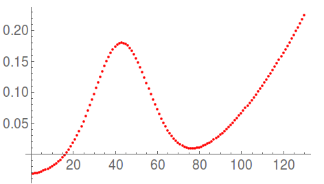
sol2adapplot = ListPlot[sol2adap, PlotStyle -> {Red, Thick}]

enter image description here

I can see that there exist one root for this last equation and it is around 16.8 but how can I find the exact value for it ? This value is for #1 but as it becomes a numerical value with apply, I can not use FindRoot or other numerical commands for a numerical root.

I have normally two equations system which I reduce to one equation and make its graphic. I could make the graph of the reduced equation but I can not find the appropriate command to find its root. Here is the code I use (from this answer) ;

u[c_] := (c^(1 - σ) - 1)/(1 - σ)
h[s_] := (2 hbar)/(1 + Exp[η (1 - s/sbar)])
d[s_] := (b s^2)/2
k[m_] := m^α
r[m_, s_] := pricemit - (D[u[c], c] /. c -> (χ s + k[m])/β) D[k[m], m]

The calibration is as follows ;

paramFinal2 = {σ -> 2.1, ρ -> 0.01, sbar -> 50, η -> 5.8, hbar -> 0.04, b -> 0.0001, γ -> 0.6, χ -> 0.025, ω -> 0.185, δ -> 0.0015, x -> 0.0014, β -> 0.8, ζ -> 0.5, τ -> 0.5, pricemit -> 0.006, α -> 0.15};

From the equation "r", I find a different couples of $m$ and $s$ which make this equation equal to zero, with starting to give 0 for $s$ (until 130) and I find corresponding "m" values.

sol[i_] := FindRoot[r[m, i] == 0 /. paramFinal2, {m, 10}];
tab = Table[sol[i], {i, 0, 130}];
Flatten[tab];

I name these values as ;

mylist = Last /@ Flatten[Table[sol[i], {i, 1, 130}]];
mylistrange = Range[1, 130];

I write the reduced equation with command Apply and plot it after ;

sol2adap = Apply[-χ - (ρ + h[#1]) + h'[#1]/(ρ + h[#1]) ((u[χ/β #1 + k[#2]/β] - d[#1] - pricemit #2)/(u'[χ/β #1 + k[#2]/β]/β)) + d'[#1]/(u'[χ/β #1 + k[#2]/β]/β) /. paramFinal2 &, {mylistrange, mylist}];
sol2adapplot = ListPlot[sol2adap, PlotStyle -> {Red, Thick}]

enter image description here

I can see that there exist one root for this last equation and it is around 16.8 but how can I find the exact value for it ? This value is for #1 but as it becomes a numerical value with apply, I can not use FindRoot or other numerical commands for a numerical root.

added 76 characters in body; edited tags
Source Link
Dr. belisarius
  • 116.2k
  • 13
  • 205
  • 456

I have normally two equations system which I reduce to one equation and make its graphic. I could make the graph of the reduced equation but I can not find the appropriate command to find its root. Here is the code I use (from this answer) ;

u[c_] := (c^(1 - σ) - 1)/(1 - σ)
h[s_] := (2 hbar)/(1 + Exp[η (1 - s/sbar)])
d[s_] := (b s^2)/2
k[m_] := m^α
r[m_, s_] := pricemit - (D[u[c], c] /. c -> (χ s + k[m])/β) D[k[m], m]

The calibration is as follows ;

paramFinal2 = {σ -> 2.1, ρ -> 0.01, sbar -> 50, η -> 5.8, hbar -> 0.04, b -> 0.0001, γ -> 0.6, χ -> 0.025, ω -> 0.185, δ -> 0.0015, x -> 0.0014, β -> 0.8, ζ -> 0.5, τ -> 0.5, pricemit -> 0.006, α -> 0.15};

From the equation "r", I find a different couples of $m$ and $s$ which make this equation equal to zero, with starting to give 0 for $s$ (until 130) and I find corresponding "m" values.

sol[i_] := FindRoot[r[m, i] == 0 /. paramFinal2, {m, 10}];
tab = Table[sol[i], {i, 0, 130}];
Flatten[tab];

I name these values as ;

mylist = Last /@ Flatten[Table[sol[i], {i, 1, 130}]];
mylistrange = Range[1, 130];

I write the reduced equation with command Apply and plot it after ;

sol2adap = Apply[-χ - (ρ + h[#1]) + h'[#1]/(ρ + h[#1]) ((u[χ/β #1 + k[#2]/β] - d[#1] - pricemit #2)/(u'[χ/β #1 + k[#2]/β]/β)) + d'[#1]/(u'[χ/β #1 + k[#2]/β]/β) /. paramFinal2 &, {mylistrange, mylist}];
sol2adapplot = ListPlot[sol2adap, PlotStyle -> {Red, Thick}]

enter image description here

I can see that there exist one root for this last equation and it is around 16.8 but how can I find the exact value for it ? This value is for #1 but as it becomes a numerical value with apply, I can not use FindRoot or other numerical commands for a numerical root.

I have normally two equations system which I reduce to one equation and make its graphic. I could make the graph of the reduced equation but I can not find the appropriate command to find its root. Here is the code I use ;

u[c_] := (c^(1 - σ) - 1)/(1 - σ)
h[s_] := (2 hbar)/(1 + Exp[η (1 - s/sbar)])
d[s_] := (b s^2)/2
k[m_] := m^α
r[m_, s_] := pricemit - (D[u[c], c] /. c -> (χ s + k[m])/β) D[k[m], m]

The calibration is as follows ;

paramFinal2 = {σ -> 2.1, ρ -> 0.01, sbar -> 50, η -> 5.8, hbar -> 0.04, b -> 0.0001, γ -> 0.6, χ -> 0.025, ω -> 0.185, δ -> 0.0015, x -> 0.0014, β -> 0.8, ζ -> 0.5, τ -> 0.5, pricemit -> 0.006, α -> 0.15};

From the equation "r", I find a different couples of $m$ and $s$ which make this equation equal to zero, with starting to give 0 for $s$ (until 130) and I find corresponding "m" values.

sol[i_] := FindRoot[r[m, i] == 0 /. paramFinal2, {m, 10}];
tab = Table[sol[i], {i, 0, 130}];
Flatten[tab];

I name these values as ;

mylist = Last /@ Flatten[Table[sol[i], {i, 1, 130}]];
mylistrange = Range[1, 130];

I write the reduced equation with command Apply and plot it after ;

sol2adap = Apply[-χ - (ρ + h[#1]) + h'[#1]/(ρ + h[#1]) ((u[χ/β #1 + k[#2]/β] - d[#1] - pricemit #2)/(u'[χ/β #1 + k[#2]/β]/β)) + d'[#1]/(u'[χ/β #1 + k[#2]/β]/β) /. paramFinal2 &, {mylistrange, mylist}];
sol2adapplot = ListPlot[sol2adap, PlotStyle -> {Red, Thick}]

enter image description here

I can see that there exist one root for this last equation and it is around 16.8 but how can I find the exact value for it ? This value is for #1 but as it becomes a numerical value with apply, I can not use FindRoot or other numerical commands for a numerical root.

I have normally two equations system which I reduce to one equation and make its graphic. I could make the graph of the reduced equation but I can not find the appropriate command to find its root. Here is the code I use (from this answer) ;

u[c_] := (c^(1 - σ) - 1)/(1 - σ)
h[s_] := (2 hbar)/(1 + Exp[η (1 - s/sbar)])
d[s_] := (b s^2)/2
k[m_] := m^α
r[m_, s_] := pricemit - (D[u[c], c] /. c -> (χ s + k[m])/β) D[k[m], m]

The calibration is as follows ;

paramFinal2 = {σ -> 2.1, ρ -> 0.01, sbar -> 50, η -> 5.8, hbar -> 0.04, b -> 0.0001, γ -> 0.6, χ -> 0.025, ω -> 0.185, δ -> 0.0015, x -> 0.0014, β -> 0.8, ζ -> 0.5, τ -> 0.5, pricemit -> 0.006, α -> 0.15};

From the equation "r", I find a different couples of $m$ and $s$ which make this equation equal to zero, with starting to give 0 for $s$ (until 130) and I find corresponding "m" values.

sol[i_] := FindRoot[r[m, i] == 0 /. paramFinal2, {m, 10}];
tab = Table[sol[i], {i, 0, 130}];
Flatten[tab];

I name these values as ;

mylist = Last /@ Flatten[Table[sol[i], {i, 1, 130}]];
mylistrange = Range[1, 130];

I write the reduced equation with command Apply and plot it after ;

sol2adap = Apply[-χ - (ρ + h[#1]) + h'[#1]/(ρ + h[#1]) ((u[χ/β #1 + k[#2]/β] - d[#1] - pricemit #2)/(u'[χ/β #1 + k[#2]/β]/β)) + d'[#1]/(u'[χ/β #1 + k[#2]/β]/β) /. paramFinal2 &, {mylistrange, mylist}];
sol2adapplot = ListPlot[sol2adap, PlotStyle -> {Red, Thick}]

enter image description here

I can see that there exist one root for this last equation and it is around 16.8 but how can I find the exact value for it ? This value is for #1 but as it becomes a numerical value with apply, I can not use FindRoot or other numerical commands for a numerical root.

deleted 91 characters in body
Source Link
Jason B.
  • 70.2k
  • 3
  • 144
  • 297

I have normally two equations system which I reduce to one equation and make its graphic. I could make the graph of the reduced equation but I can not find the appropriate command to find its root. Here is the code I use ;

u[c_] := (c^(1 - \[Sigma]σ) - 1)/(1 - \[Sigma]σ)
h[s_] := (2 hbar)/(1 + Exp[\[Eta]Exp[η (1 - s/sbar)])
d[s_] := (b s^2)/2
k[m_] := m^\[Alpha]m^α
r[m_, s_] := pricemit - (D[u[c], c] /. c -> (\[Chi]χ s + k[m])/\[Beta]β) D[k[m], m]

The calibration is as follows ;

paramFinal2 = {\[Sigma]σ -> 2.1, \[Rho]ρ -> 0.01, sbar -> 50, \[Eta]η -> 5.8, hbar -> 0.04, b -> 0.0001, \[Gamma]γ -> 0.6, \[Chi]χ -> 0.025, \[Omega]ω -> 0.185, \[Delta]δ -> 0.0015, x -> 0.0014, \[Beta]β -> 0.8, \[Zeta]ζ -> 0.5, \[Tau]τ -> 0.5, pricemit -> 0.006, \[Alpha]α -> 0.15};

From the equation "r", I find a different couples of $m$ and $s$ which make this equation equal to zero, with starting to give 0 for $s$ (until 130) and I find corresponding "m" values.

sol[i_] := FindRoot[r[m, i] == 0 /. paramFinal2, {m, 10}];
tab = Table[sol[i], {i, 0, 130}];
Flatten[tab];

I name these values as ;

mylist = Last /@ Flatten[Table[sol[i], {i, 1, 130}]];
mylistrange = Range[1, 130];

I write the reduced equation with command Apply and plot it after ;

sol2adap = Apply[-\[Chi]χ - (\[Rho]ρ + h[#1]) + h'[#1]/(\[Rho]ρ + h[#1]) ((u[\[Chi]u[χ/\[Beta]β #1 + k[#2]/\[Beta]]β] - d[#1] - pricemit #2)/(u'[\[Chi]u'[χ/\[Beta]β #1 + k[#2]/[Beta]]β]/\[Beta]β)) + d'[#1]/(u'[\[Chi]u'[χ/\[Beta]β #1 + k[#2]/\[Beta]]β]/\[Beta]β) /. paramFinal2 &, {mylistrange, mylist}];
sol2adapplot = ListPlot[sol2adap, PlotStyle -> {Red, Thick}]

enter image description here

I can see that there exist one root for this last equation and it is around 16.8 but how can I find the exact value for it ? This value is for #1 but as it becomes a numerical value with apply, I can not use FindRoot or other numerical commands for a numerical root.

I have normally two equations system which I reduce to one equation and make its graphic. I could make the graph of the reduced equation but I can not find the appropriate command to find its root. Here is the code I use ;

u[c_] := (c^(1 - \[Sigma]) - 1)/(1 - \[Sigma])
h[s_] := (2 hbar)/(1 + Exp[\[Eta] (1 - s/sbar)])
d[s_] := (b s^2)/2
k[m_] := m^\[Alpha]
r[m_, s_] := pricemit - (D[u[c], c] /. c -> (\[Chi] s + k[m])/\[Beta]) D[k[m], m]

The calibration is as follows ;

paramFinal2 = {\[Sigma] -> 2.1, \[Rho] -> 0.01, sbar -> 50, \[Eta] -> 5.8, hbar -> 0.04, b -> 0.0001, \[Gamma] -> 0.6, \[Chi] -> 0.025, \[Omega] -> 0.185, \[Delta] -> 0.0015, x -> 0.0014, \[Beta] -> 0.8, \[Zeta] -> 0.5, \[Tau] -> 0.5, pricemit -> 0.006, \[Alpha] -> 0.15};

From the equation "r", I find a different couples of $m$ and $s$ which make this equation equal to zero, with starting to give 0 for $s$ (until 130) and I find corresponding "m" values.

sol[i_] := FindRoot[r[m, i] == 0 /. paramFinal2, {m, 10}];
tab = Table[sol[i], {i, 0, 130}];
Flatten[tab];

I name these values as ;

mylist = Last /@ Flatten[Table[sol[i], {i, 1, 130}]];
mylistrange = Range[1, 130];

I write the reduced equation with command Apply and plot it after ;

sol2adap = Apply[-\[Chi] - (\[Rho] + h[#1]) + h'[#1]/(\[Rho] + h[#1]) ((u[\[Chi]/\[Beta] #1 + k[#2]/\[Beta]] - d[#1] - pricemit #2)/(u'[\[Chi]/\[Beta] #1 + k[#2]/[Beta]]/\[Beta])) + d'[#1]/(u'[\[Chi]/\[Beta] #1 + k[#2]/\[Beta]]/\[Beta]) /. paramFinal2 &, {mylistrange, mylist}];
sol2adapplot = ListPlot[sol2adap, PlotStyle -> {Red, Thick}]

I can see that there exist one root for this last equation and it is around 16.8 but how can I find the exact value for it ? This value is for #1 but as it becomes a numerical value with apply, I can not use FindRoot or other numerical commands for a numerical root.

I have normally two equations system which I reduce to one equation and make its graphic. I could make the graph of the reduced equation but I can not find the appropriate command to find its root. Here is the code I use ;

u[c_] := (c^(1 - σ) - 1)/(1 - σ)
h[s_] := (2 hbar)/(1 + Exp[η (1 - s/sbar)])
d[s_] := (b s^2)/2
k[m_] := m^α
r[m_, s_] := pricemit - (D[u[c], c] /. c -> (χ s + k[m])/β) D[k[m], m]

The calibration is as follows ;

paramFinal2 = {σ -> 2.1, ρ -> 0.01, sbar -> 50, η -> 5.8, hbar -> 0.04, b -> 0.0001, γ -> 0.6, χ -> 0.025, ω -> 0.185, δ -> 0.0015, x -> 0.0014, β -> 0.8, ζ -> 0.5, τ -> 0.5, pricemit -> 0.006, α -> 0.15};

From the equation "r", I find a different couples of $m$ and $s$ which make this equation equal to zero, with starting to give 0 for $s$ (until 130) and I find corresponding "m" values.

sol[i_] := FindRoot[r[m, i] == 0 /. paramFinal2, {m, 10}];
tab = Table[sol[i], {i, 0, 130}];
Flatten[tab];

I name these values as ;

mylist = Last /@ Flatten[Table[sol[i], {i, 1, 130}]];
mylistrange = Range[1, 130];

I write the reduced equation with command Apply and plot it after ;

sol2adap = Apply[-χ - (ρ + h[#1]) + h'[#1]/(ρ + h[#1]) ((u[χ/β #1 + k[#2]/β] - d[#1] - pricemit #2)/(u'[χ/β #1 + k[#2]/β]/β)) + d'[#1]/(u'[χ/β #1 + k[#2]/β]/β) /. paramFinal2 &, {mylistrange, mylist}];
sol2adapplot = ListPlot[sol2adap, PlotStyle -> {Red, Thick}]

enter image description here

I can see that there exist one root for this last equation and it is around 16.8 but how can I find the exact value for it ? This value is for #1 but as it becomes a numerical value with apply, I can not use FindRoot or other numerical commands for a numerical root.

added 114 characters in body
Source Link
Loading
Source Link
Loading