We wish to find $y(x)$ such that $f(x,y(x)) = 0$. We know that $f(0,0) = 0$; thus, $y(0) = 0$. We also know that if $f(x,y(x)) = 0$, then $$ \frac{d}{dx} f(x,y(x)) = 0 $$ as well. Thus, we can replace the condition $f(x,y(x)) = 0$ with the conditions $$ \frac{d}{dx} f(x,y(x)) = 0, \qquad y(0) = 0. $$ These two equations are a first-order differential equation in $y(x)$, and an "initial condition" for $y(x)$. It's still not exactly soluble, but NDSolve can handle it numerically and return an InterpolatingFunction solution. You can then feed your desired values of x into the InterpolatingFunction using Map to get a corresponding table of $y$-values.

Implemented:

f[x_, y_] = Sinh[y] - (y + Tanh[x]) Cosh[y] - y Sech[x]^2;
soln = NDSolve[{y[0] == 0, D[f[x, y[x]], x] == 0}, y, {x, -5, 5}];
xList = Array[# &, 10000, {-5, 5}];
yList = First[y /. soln] /@ xList

This method has the advantage of not calling a numerical root-finder such as FindRoot or Solve 10,000 times, and so is pretty fast. On my machine, I get a result within about 40 milliseconds.

If you want to plot it, you can do that too:

Plot[y[x] /. soln, {x, -5, 5}]

Note that this method relies on the fact that (a) there was only one connected contour of $f(x,y) = 0$, (b) it led to a well-defined function $y(x)$, as opposed to multiple $y$-values corresponding to a single $x$, and (c) we knew a point that it passed through, namely $(0,0)$. If you picked another $f$ you might not have such luck. Condition (c) would be easy enough to relax (a FindInstance call would probably give you a starting point for your initial conditions), but (a) and (b) would be harder to get around.

We wish to find $y(x)$ such that $f(x,y(x)) = 0$. We know that $f(0,0) = 0$; thus, $y(0) = 0$. We also know that if $f(x,y(x)) = 0$, then $$ \frac{d}{dx} f(x,y(x)) = 0 $$ as well. Thus, we can replace the condition $f(x,y(x)) = 0$ with the conditions $$ \frac{d}{dx} f(x,y(x)) = 0, \qquad y(0) = 0. $$ These two equations are a first-order differential equation in $y(x)$, and an "initial condition" for $y(x)$. It's still not exactly soluble, but NDSolve can handle it numerically and return an InterpolatingFunction solution. You can then feed your desired values of x into the InterpolatingFunction using Map to get a corresponding table of $y$-values.

Implemented:

f[x_, y_] = Sinh[y] - (y + Tanh[x]) Cosh[y] - y Sech[x]^2;
soln = NDSolve[{y[0] == 0, D[f[x, y[x]], x] == 0}, y, {x, -5, 5}];
xList = Array[# &, 10000, {-5, 5}];
yList = First[y /. soln] /@ xList

This method has the advantage of not calling a numerical root-finder such as FindRoot or Solve 10,000 times, and so is pretty fast. On my machine, I get a result within about 40 milliseconds.

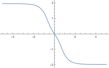
If you want to plot it, you can do that too:

Plot[y[x] /. soln, {x, -5, 5}]

Note that this method relies on three facts:

1. there was only one connected contour of $f(x,y) = 0$,
2. it led to a well-defined function $y(x)$, as opposed to multiple $y$-values corresponding to a single $x$, and
3. we knew a point that it passed through, namely $(0,0)$.

If you picked another $f$ you might not have such luck. Condition 3 would be easy enough to relax (a FindInstance call would probably give you a starting point for your initial conditions), but Conditions 1 and 2 would be harder to get around.

We wish to find $y(x)$ such that $f(x,y(x)) = 0$. We know that $f(0,0) = 0$; thus, $y(0) = 0$. We also know that if $f(x,y(x)) = 0$, then $$ \frac{d}{dx} f(x,y(x)) = 0 $$ as well. Thus, we can replace the condition $f(x,y(x)) = 0$ with the conditions $$ \frac{d}{dx} f(x,y(x)) = 0, \qquad y(0) = 0. $$ These two equations are a first-order differential equation in $y(x)$, and an "initial condition" for $y(x)$. It's still not exactly soluble, but NDSolve can handle it numerically and return an InterpolatingFunction solution. You can then feed your desired values of x into the InterpolatingFunction using Map to get a corresponding table of $y$-values.

Implemented:

f[x_, y_] = Sinh[y] - (y + Tanh[x]) Cosh[y] - y Sech[x]^2;
soln = NDSolve[{y[0] == 0, D[f[x, y[x]], x] == 0}, y, {x, -5, 5}];
xList = Array[# &, 10000, {-5, 5}];
yList = First[y /. soln] /@ xList

This method has the advantage of not calling a numerical root-finder such as FindRoot or Solve 10,000 times, and so is pretty fast. On my machine, I get a result within about 40 milliseconds.

Note that this will only give you a function $y(x)$ corresponding to the contour of $f(x,y) = 0$ that passes through $(0,0)$. This appears to be the only such contour in this case, but if you picked another $f$ you might not have such luck.

We wish to find $y(x)$ such that $f(x,y(x)) = 0$. We know that $f(0,0) = 0$; thus, $y(0) = 0$. We also know that if $f(x,y(x)) = 0$, then $$ \frac{d}{dx} f(x,y(x)) = 0 $$ as well. Thus, we can replace the condition $f(x,y(x)) = 0$ with the conditions $$ \frac{d}{dx} f(x,y(x)) = 0, \qquad y(0) = 0. $$ These two equations are a first-order differential equation in $y(x)$, and an "initial condition" for $y(x)$. It's still not exactly soluble, but NDSolve can handle it numerically and return an InterpolatingFunction solution. You can then feed your desired values of x into the InterpolatingFunction using Map to get a corresponding table of $y$-values.

Implemented:

f[x_, y_] = Sinh[y] - (y + Tanh[x]) Cosh[y] - y Sech[x]^2;
soln = NDSolve[{y[0] == 0, D[f[x, y[x]], x] == 0}, y, {x, -5, 5}];
xList = Array[# &, 10000, {-5, 5}];
yList = First[y /. soln] /@ xList

This method has the advantage of not calling a numerical root-finder such as FindRoot or Solve 10,000 times, and so is pretty fast. On my machine, I get a result within about 40 milliseconds.

If you want to plot it, you can do that too:

Plot[y[x] /. soln, {x, -5, 5}]

Note that this method relies on the fact that (a) there was only one connected contour of $f(x,y) = 0$, (b) it led to a well-defined function $y(x)$, as opposed to multiple $y$-values corresponding to a single $x$, and (c) we knew a point that it passed through, namely $(0,0)$. If you picked another $f$ you might not have such luck. Condition (c) would be easy enough to relax (a FindInstance call would probably give you a starting point for your initial conditions), but (a) and (b) would be harder to get around.