edited body
Source Link
Greg Hurst
  • 36.8k
  • 1
  • 94
  • 143

Here's one where we treat the abdomen differently.

First, look at this as a 2D parametric curve:

r[t_] := E^Sin[t] - 24/10 Cos[4 t] + Sin[t/12]
x[t_] := r[t] Cos[t]
y[t_] := r[t] Sin[t]

We can locate the abdomen by carefully partitioning the roots of x[t].

vals = First[Cases[Plot[Evaluate[x[t, 0]], {t, 0, 20π}], Line[l_] :> l, ∞]];

xroots = t /. FindRoot[x[t], {t, ##}, WorkingPrecision -> 30] & @@@
 Select[Partition[vals, 2, 1], Sign[#[[1, 2]]] != Sign[#[[2, 2]]] &][[All, All, 1]];

We now will define the abdomen through inequalities of our parameter t.

AbdomenQ[r_] := With[{s = Chop@y[r]},
  s < 0 || (s > 1 && s > Chop@y[r - 1/100])
]

abdomenextrema = Select[xroots, AbdomenQ];

abdomen = N[Or @@ (#1 <= t <= #3 & @@@ 
  Cases[Partition[xroots, 3, 1], {_, Alternatives @@ abdomenextrema, _}])];

Now when we define our 3D parametric equation, we need to make sure our point rotates if and only if it's on a wing.

r[t_] := E^Sin[t] - 24/10 Cos[4 t] + Sin[t/12]
(x[t_, a_] := If[#, r[u]r[t] Cos[t], r[t] Cos[t] Cos[a]]) &[abdomen]
y[t_, a_] := r[t] Sin[t]
(z[t_, a_] := If[#, 0., Sign[a] Abs[r[t] Cos[t] Sin[a]]])&[abdomen]

We also keep the abdomen black and make the wings colorful.

cf = Function[{x, y, z, t}, 
  If[#,
    Black,
    #2[Sqrt[x^2 + y^2]/6]
  ]
]&[abdomen, ColorData["FruitPunchColors"]];

And now we place this in a nicely formatted Animate.

Animate[ParametricPlot3D[{x[t, a], y[t, a], z[t, a]}, {t, 0, 20π}, 
   PlotRange -> 8 {{-1, 1}, {-1, 1}, {-1, 1}}, 
   PlotPoints -> ControlActive[100, Automatic], 
   ColorFunction -> cf, 
   ColorFunctionScaling -> False, 
   Boxed -> False, 
   Axes -> False
  ], 
  {{a, 0.001}, -Pi/6, Pi/2}, 
  AnimationDirection -> ForwardBackward, 
  AnimationRate -> 1
]

enter image description here

Here's one where we treat the abdomen differently.

First, look at this as a 2D parametric curve:

r[t_] := E^Sin[t] - 24/10 Cos[4 t] + Sin[t/12]
x[t_] := r[t] Cos[t]
y[t_] := r[t] Sin[t]

We can locate the abdomen by carefully partitioning the roots of x[t].

vals = First[Cases[Plot[Evaluate[x[t, 0]], {t, 0, 20π}], Line[l_] :> l, ∞]];

xroots = t /. FindRoot[x[t], {t, ##}, WorkingPrecision -> 30] & @@@
 Select[Partition[vals, 2, 1], Sign[#[[1, 2]]] != Sign[#[[2, 2]]] &][[All, All, 1]];

We now will define the abdomen through inequalities of our parameter t.

AbdomenQ[r_] := With[{s = Chop@y[r]},
  s < 0 || (s > 1 && s > Chop@y[r - 1/100])
]

abdomenextrema = Select[xroots, AbdomenQ];

abdomen = N[Or @@ (#1 <= t <= #3 & @@@ 
  Cases[Partition[xroots, 3, 1], {_, Alternatives @@ abdomenextrema, _}])];

Now when we define our 3D parametric equation, we need to make sure our point rotates if and only if it's on a wing.

r[t_] := E^Sin[t] - 24/10 Cos[4 t] + Sin[t/12]
(x[t_, a_] := If[#, r[u] Cos[t], r[t] Cos[t] Cos[a]]) &[abdomen]
y[t_, a_] := r[t] Sin[t]
(z[t_, a_] := If[#, 0., Sign[a] Abs[r[t] Cos[t] Sin[a]]])&[abdomen]

We also keep the abdomen black and make the wings colorful.

cf = Function[{x, y, z, t}, 
  If[#,
    Black,
    #2[Sqrt[x^2 + y^2]/6]
  ]
]&[abdomen, ColorData["FruitPunchColors"]];

And now we place this in a nicely formatted Animate.

Animate[ParametricPlot3D[{x[t, a], y[t, a], z[t, a]}, {t, 0, 20π}, 
   PlotRange -> 8 {{-1, 1}, {-1, 1}, {-1, 1}}, 
   PlotPoints -> ControlActive[100, Automatic], 
   ColorFunction -> cf, 
   ColorFunctionScaling -> False, 
   Boxed -> False, 
   Axes -> False
  ], 
  {{a, 0.001}, -Pi/6, Pi/2}, 
  AnimationDirection -> ForwardBackward, 
  AnimationRate -> 1
]
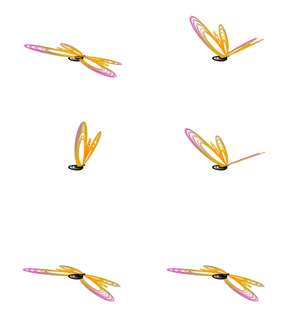
enter image description here

Here's one where we treat the abdomen differently.

First, look at this as a 2D parametric curve:

r[t_] := E^Sin[t] - 24/10 Cos[4 t] + Sin[t/12]
x[t_] := r[t] Cos[t]
y[t_] := r[t] Sin[t]

We can locate the abdomen by carefully partitioning the roots of x[t].

vals = First[Cases[Plot[Evaluate[x[t, 0]], {t, 0, 20π}], Line[l_] :> l, ∞]];

xroots = t /. FindRoot[x[t], {t, ##}, WorkingPrecision -> 30] & @@@
 Select[Partition[vals, 2, 1], Sign[#[[1, 2]]] != Sign[#[[2, 2]]] &][[All, All, 1]];

We now will define the abdomen through inequalities of our parameter t.

AbdomenQ[r_] := With[{s = Chop@y[r]},
  s < 0 || (s > 1 && s > Chop@y[r - 1/100])
]

abdomenextrema = Select[xroots, AbdomenQ];

abdomen = N[Or @@ (#1 <= t <= #3 & @@@ 
  Cases[Partition[xroots, 3, 1], {_, Alternatives @@ abdomenextrema, _}])];

Now when we define our 3D parametric equation, we need to make sure our point rotates if and only if it's on a wing.

r[t_] := E^Sin[t] - 24/10 Cos[4 t] + Sin[t/12]
(x[t_, a_] := If[#, r[t] Cos[t], r[t] Cos[t] Cos[a]]) &[abdomen]
y[t_, a_] := r[t] Sin[t]
(z[t_, a_] := If[#, 0., Sign[a] Abs[r[t] Cos[t] Sin[a]]])&[abdomen]

We also keep the abdomen black and make the wings colorful.

cf = Function[{x, y, z, t}, 
  If[#,
    Black,
    #2[Sqrt[x^2 + y^2]/6]
  ]
]&[abdomen, ColorData["FruitPunchColors"]];

And now we place this in a nicely formatted Animate.

Animate[ParametricPlot3D[{x[t, a], y[t, a], z[t, a]}, {t, 0, 20π}, 
   PlotRange -> 8 {{-1, 1}, {-1, 1}, {-1, 1}}, 
   PlotPoints -> ControlActive[100, Automatic], 
   ColorFunction -> cf, 
   ColorFunctionScaling -> False, 
   Boxed -> False, 
   Axes -> False
  ], 
  {{a, 0.001}, -Pi/6, Pi/2}, 
  AnimationDirection -> ForwardBackward, 
  AnimationRate -> 1
]

enter image description here

deleted 6 characters in body
Source Link
Greg Hurst
  • 36.8k
  • 1
  • 94
  • 143

Here's one where we treat the abdomen differently.

First, look at this as a 2D parametric curve:

r[t_] := E^Sin[t] - 24/10 Cos[4 t] + Sin[t/12]
x[t_] := r[t] Cos[t]
y[t_] := r[t] Sin[t]

We can locate the abdomen by carefully partitioning the roots of x[t].

vals = First[Cases[Plot[Evaluate[x[t, 0]], {t, 0, 20π}], Line[l_] :> l, ∞]];

xroots = t /. FindRoot[x[t], {t, ##}, WorkingPrecision -> 30] & @@@
 Select[Partition[vals, 2, 1], Sign[#[[1, 2]]] != Sign[#[[2, 2]]] &][[All, All, 1]];

We now will define the abdomen through inequalities of our parameter t.

AbdomenQ[r_] := With[{s = Chop@y[r, 0]Chop@y[r]},
  s < 0 || (s > 1 && s > Chop@y[r - 1/100, 0]100])
]

abdomenextrema = Select[xroots, AbdomenQ];

abdomen = N[Or @@ (#1 <= t <= #3 & @@@ 
  Cases[Partition[xroots, 3, 1], {_, Alternatives @@ abdomenextrema, _}])];

Now when we define our 3D parametric equation, we need to make sure our point rotates if and only if it's on a wing.

r[t_] := E^Sin[t] - 24/10 Cos[4 t] + Sin[t/12]
(x[t_, a_] := If[#, r[u] Cos[t], r[t] Cos[t] Cos[a]]) &[abdomen]
y[t_, a_] := r[t] Sin[t]
(z[t_, a_] := If[#, 0., Sign[a] Abs[r[t] Cos[t] Sin[a]]])&[abdomen]

We also keep the abdomen black and make the wings colorful.

cf = Function[{x, y, z, t}, 
  If[#,
    Black,
    #2[Sqrt[x^2 + y^2]/6]
  ]
]&[abdomen, ColorData["FruitPunchColors"]];

And now we place this in a nicely formatted Animate.

Animate[ParametricPlot3D[{x[t, a], y[t, a], z[t, a]}, {t, 0, 20π}, 
   PlotRange -> 8 {{-1, 1}, {-1, 1}, {-1, 1}}, 
   PlotPoints -> ControlActive[100, Automatic], 
   ColorFunction -> cf, 
   ColorFunctionScaling -> False, 
   Boxed -> False, 
   Axes -> False
  ], 
  {{a, 0.001}, -Pi/6, Pi/2}, 
  AnimationDirection -> ForwardBackward, 
  AnimationRate -> 1
]

enter image description here

Here's one where we treat the abdomen differently.

First, look at this as a 2D parametric curve:

r[t_] := E^Sin[t] - 24/10 Cos[4 t] + Sin[t/12]
x[t_] := r[t] Cos[t]
y[t_] := r[t] Sin[t]

We can locate the abdomen by carefully partitioning the roots of x[t].

vals = First[Cases[Plot[Evaluate[x[t, 0]], {t, 0, 20π}], Line[l_] :> l, ∞]];

xroots = t /. FindRoot[x[t], {t, ##}, WorkingPrecision -> 30] & @@@
 Select[Partition[vals, 2, 1], Sign[#[[1, 2]]] != Sign[#[[2, 2]]] &][[All, All, 1]];

We now will define the abdomen through inequalities of our parameter t.

AbdomenQ[r_] := With[{s = Chop@y[r, 0]},
  s < 0 || (s > 1 && s > Chop@y[r - 1/100, 0])
]

abdomenextrema = Select[xroots, AbdomenQ];

abdomen = N[Or @@ (#1 <= t <= #3 & @@@ 
  Cases[Partition[xroots, 3, 1], {_, Alternatives @@ abdomenextrema, _}])];

Now when we define our 3D parametric equation, we need to make sure our point rotates if and only if it's on a wing.

r[t_] := E^Sin[t] - 24/10 Cos[4 t] + Sin[t/12]
(x[t_, a_] := If[#, r[u] Cos[t], r[t] Cos[t] Cos[a]]) &[abdomen]
y[t_, a_] := r[t] Sin[t]
(z[t_, a_] := If[#, 0., Sign[a] Abs[r[t] Cos[t] Sin[a]]])&[abdomen]

We also keep the abdomen black and make the wings colorful.

cf = Function[{x, y, z, t}, 
  If[#,
    Black,
    #2[Sqrt[x^2 + y^2]/6]
  ]
]&[abdomen, ColorData["FruitPunchColors"]];

And now we place this in a nicely formatted Animate.

Animate[ParametricPlot3D[{x[t, a], y[t, a], z[t, a]}, {t, 0, 20π}, 
   PlotRange -> 8 {{-1, 1}, {-1, 1}, {-1, 1}}, 
   PlotPoints -> ControlActive[100, Automatic], 
   ColorFunction -> cf, 
   ColorFunctionScaling -> False, 
   Boxed -> False, 
   Axes -> False
  ], 
  {{a, 0.001}, -Pi/6, Pi/2}, 
  AnimationDirection -> ForwardBackward, 
  AnimationRate -> 1
]

enter image description here

Here's one where we treat the abdomen differently.

First, look at this as a 2D parametric curve:

r[t_] := E^Sin[t] - 24/10 Cos[4 t] + Sin[t/12]
x[t_] := r[t] Cos[t]
y[t_] := r[t] Sin[t]

We can locate the abdomen by carefully partitioning the roots of x[t].

vals = First[Cases[Plot[Evaluate[x[t, 0]], {t, 0, 20π}], Line[l_] :> l, ∞]];

xroots = t /. FindRoot[x[t], {t, ##}, WorkingPrecision -> 30] & @@@
 Select[Partition[vals, 2, 1], Sign[#[[1, 2]]] != Sign[#[[2, 2]]] &][[All, All, 1]];

We now will define the abdomen through inequalities of our parameter t.

AbdomenQ[r_] := With[{s = Chop@y[r]},
  s < 0 || (s > 1 && s > Chop@y[r - 1/100])
]

abdomenextrema = Select[xroots, AbdomenQ];

abdomen = N[Or @@ (#1 <= t <= #3 & @@@ 
  Cases[Partition[xroots, 3, 1], {_, Alternatives @@ abdomenextrema, _}])];

Now when we define our 3D parametric equation, we need to make sure our point rotates if and only if it's on a wing.

r[t_] := E^Sin[t] - 24/10 Cos[4 t] + Sin[t/12]
(x[t_, a_] := If[#, r[u] Cos[t], r[t] Cos[t] Cos[a]]) &[abdomen]
y[t_, a_] := r[t] Sin[t]
(z[t_, a_] := If[#, 0., Sign[a] Abs[r[t] Cos[t] Sin[a]]])&[abdomen]

We also keep the abdomen black and make the wings colorful.

cf = Function[{x, y, z, t}, 
  If[#,
    Black,
    #2[Sqrt[x^2 + y^2]/6]
  ]
]&[abdomen, ColorData["FruitPunchColors"]];

And now we place this in a nicely formatted Animate.

Animate[ParametricPlot3D[{x[t, a], y[t, a], z[t, a]}, {t, 0, 20π}, 
   PlotRange -> 8 {{-1, 1}, {-1, 1}, {-1, 1}}, 
   PlotPoints -> ControlActive[100, Automatic], 
   ColorFunction -> cf, 
   ColorFunctionScaling -> False, 
   Boxed -> False, 
   Axes -> False
  ], 
  {{a, 0.001}, -Pi/6, Pi/2}, 
  AnimationDirection -> ForwardBackward, 
  AnimationRate -> 1
]

enter image description here

Source Link
Greg Hurst
  • 36.8k
  • 1
  • 94
  • 143

Here's one where we treat the abdomen differently.

First, look at this as a 2D parametric curve:

r[t_] := E^Sin[t] - 24/10 Cos[4 t] + Sin[t/12]
x[t_] := r[t] Cos[t]
y[t_] := r[t] Sin[t]

We can locate the abdomen by carefully partitioning the roots of x[t].

vals = First[Cases[Plot[Evaluate[x[t, 0]], {t, 0, 20π}], Line[l_] :> l, ∞]];

xroots = t /. FindRoot[x[t], {t, ##}, WorkingPrecision -> 30] & @@@
 Select[Partition[vals, 2, 1], Sign[#[[1, 2]]] != Sign[#[[2, 2]]] &][[All, All, 1]];

We now will define the abdomen through inequalities of our parameter t.

AbdomenQ[r_] := With[{s = Chop@y[r, 0]},
  s < 0 || (s > 1 && s > Chop@y[r - 1/100, 0])
]

abdomenextrema = Select[xroots, AbdomenQ];

abdomen = N[Or @@ (#1 <= t <= #3 & @@@ 
  Cases[Partition[xroots, 3, 1], {_, Alternatives @@ abdomenextrema, _}])];

Now when we define our 3D parametric equation, we need to make sure our point rotates if and only if it's on a wing.

r[t_] := E^Sin[t] - 24/10 Cos[4 t] + Sin[t/12]
(x[t_, a_] := If[#, r[u] Cos[t], r[t] Cos[t] Cos[a]]) &[abdomen]
y[t_, a_] := r[t] Sin[t]
(z[t_, a_] := If[#, 0., Sign[a] Abs[r[t] Cos[t] Sin[a]]])&[abdomen]

We also keep the abdomen black and make the wings colorful.

cf = Function[{x, y, z, t}, 
  If[#,
    Black,
    #2[Sqrt[x^2 + y^2]/6]
  ]
]&[abdomen, ColorData["FruitPunchColors"]];

And now we place this in a nicely formatted Animate.

Animate[ParametricPlot3D[{x[t, a], y[t, a], z[t, a]}, {t, 0, 20π}, 
   PlotRange -> 8 {{-1, 1}, {-1, 1}, {-1, 1}}, 
   PlotPoints -> ControlActive[100, Automatic], 
   ColorFunction -> cf, 
   ColorFunctionScaling -> False, 
   Boxed -> False, 
   Axes -> False
  ], 
  {{a, 0.001}, -Pi/6, Pi/2}, 
  AnimationDirection -> ForwardBackward, 
  AnimationRate -> 1
]

enter image description here