AceGen/AceFEM Explicit Meshless

Question

Hello fellow Ace Users.

Currently I'm working on a project to implement Peridynamics. This is a discretization technique in the fashion of a meshless particle method. AceGen/AceFEM provides the feature of arbitrary nodes per element which suits my need perfectly as such a peridynamic particle interacts with arbitrary number of neighbour particles. To use the benefits of this method such as modelling discontinuities I'm aiming to utilize an explicit solution procedure.

I appreciate any thoughts on this! I have some code running in AceGen/AceFEM so far, still struggling on some design decisions which lead to the following specific questions:

• 1. Whats exactly prarallelized in AceFEM? My recent experience indicate that SMSStandardModule["Tasks"] is not. Is that correct ? How about SMSStandardModule["Tangent and residual"] (I'm talking about the evaluation of the elements not solving the global equation system in parallel.)?
• 2. Is there any known (maybe approximate) limit to the performance regarding arbitrary nodes per element?
• 3. Does anyone have experiences with explicit simulations in AceFEM/AceGen?
• 4. I expect a lot of data due to the particle discretization. Visualisation in post processing will be a to hard task to do in Mathematica. Does anyone have experiences with exporting the simulation data for use in e.g Paraview? If so, what's most performant way to write these to a file without significantly slowing down the simulation? I'm aware of the SMTPut[] feature by the way, but to my knowledge this binds me to Mathematica again.

As always You have my kudos in advance and I'm excited for your comments and answers !

Thanks for the response so far.

I'm back with a 'minimal' example that shows my main concerns.

The code is provided in SimpePDImplementation on GitHub:

The element contains a vary basic implementation of explicit peridynamics following two steps for each time step:

• 1. Compute force density for each node (based on its neighbours)
• 2. Integrate in time: acceleration = force density / density (per node)

These two task are implemented twice (using the same code), for once implemented into the SKR subroutine and for once as individual element tasks. !As the code is explicit i do not want or have a system of equation to solve, but i definitely want go over all elements in parallel to gain speedup. The results for both implementations are the same as expected, however the SKR implementation run significantly slower (i guess do to the solution of the linear system which is completely zero in this case).

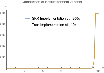
While performing the analysis, I checked my CPU usage.

For the SKR implementation I get: While for the Task implementation as reported I have:

My conclusion so far is that the parallelization only works on the solution of the linear system and at least does not parallelize the loop over all elements for tasks.

I would be great if one of you guy can confirm, or even better of course tell me what I made wrong so that I know wether AceFEM works for my purpose at all.

Best, S

Answer 1

I can mostly help with the implementation aspect of meshfree methods and answer point two. Although Mathematica can plot anything you want, but you might need to program it yourself.

2. In the new version of AceGen/FEM 6.923, prof Korelc introduced a new SMSIO functions and there is improvement of SMSArray usage and some new global fields. With that the formulation of elements with variable number of nodes is greatly simplified and the efficiency is independent of maximum number of nodes. You can put 1000 nodes if you want, the efficiency will not change more than couple %. To see the Improvement you need to introduce your vector of DOF as an array and not as a list with a fixed length of maximum possible values, additionally there are some fields that will give you actual number of nodes (I haven't tested that part). Here is a simple code extract of important things:

Function additionalNodes needs to pad actual amount of nodes with Null to match the max length for each element:

maxNodes=1000;
ClearAll[additionalNodes];

additionalNodes[nodes_, maxNodes_] := Module[{n},
   If[Length[nodes] > maxNodes,
     SMCError = {"Maximum number of nodes:", maxNodes, "Nodes:", nodes};
     SMCAbort["Given number of nodes exceeded the maximum number.", "",""];
   ];
   Join[ConstantArray[Null, maxNodes - Length[nodes]]]
];

You need to specify maximum no. of nodes, all nodes should be given as dummy-nodes and SMSAdditionalNodes should be assigned the above function:

SMSTemplate[
 "SMSTopology" -> "QX"
 , "SMSNoNodes" -> maxNodes
 , "SMSDOFGlobal" -> 2
 , "SMSNodeID" -> "D -D"
 ,...,
 , "SMSAdditionalNodes" -> Function[additionalNodes[{##},maxNodes]]
 , "SMSMMAInitialisation" -> {{Definition[additionalNodes]}, Null}
]

Inside the SMSStandardModule we can extract the actual number of nodes/DOF from a new fields (Or if you like from ed$$["Data",_] field)

nNodes ⊢ SMSLastTrueNode[];
nDOF ⊢ SMSLastTrueDOF[];
nDOFNode = SMSNoDimensions;

The vector of all unknowns can then be defined as follows with SMSArray:

pe ⊨ SMSArray[nDOF, 
 Function[{dof}, SMSIO["Nodal DOFs"[(dof - 1)/nDOFNode + 1,SMSMod[dof-1,nDOFNode] + 1]]]
];

Then we can loop over arbitrary points/edges... we can read the displacement and coordinate of each point with node defined as an SMSInteger or a loop parameter as:

XNode ⊢ Table[SMSReal[nd$$[node, "X", j]], {j, SMSNoDimensions}];
uNode ⊨ Table[SMSPart[pe, (node - 1) nDOFNode + j], {j, nDOFNode}];

After your define your potential, the Residual and tangent can be derived same way as before, but only looped over the actual no of DOF defined by nDOF:

SMSDo[Rgi ⊨ SMSD[W, pe, i, "Constant"->SMSVariables[pseudoWConstants]];
  SMSIO[Rgi, "Add to", "Residual"[i]];
  SMSDo[
    Kgij ⊨SMSD[Rgi, \[DoubleStruckP]e, j];
    SMSIO[Kgij, "Add to", "Tangent"[i, j]];
  ,{j, i, nDOF}
  ];
,{i, 1, nDOF}
];

Answer 2

I have no experience with meshless methods, but I will try to answer/comment on your questions.

1. In AceFEM assembling of global matrices and vectors ("Tangent and residual" subroutine) is parallelized. Solving the linear system is also parallelized (Intel MKL PARDISO). "Tasks" subroutine is not parallelized, but in general such procedures should not be computationally too intensive.

2. Virtual element method (VEM) has been implemented in AceGen/AceFEM and it seems many (up to 100) nodes per element are possible. See Aldakheel et. al., 2018 for example. See even better explanation in BHudobivnik answer.

3. According to comment by prof. Korelc, explicit simulations are possible. If this helps, Schmied et. al, 2013 have implemented element assembly subroutines in AceGen and used them in LS-Dyna software with explicit time integration.

4. This really depends what you would like to visualize. I would perform visualization out of Mathematica only if there was really no other option. For that purpose you can always save a limited subset of results in some efficient common data format. Maybe something like HDF? As always, I would recommend to start with small example and deal with problems of large example when/if it happens.