2
$\begingroup$

I have seen that for Riccati equation the solution can be done by

DSolve[y'[z] == P[z] + Q[z] y[z] + R[z] y[z]^2, y[z], z]

but for my case mathematica fails to compute it. I am trying this

DSolve[y'[x] + ((2.248*10^12)/x^2) (y[x])^2 - (22.48/x^2) y[x] - 
23.3455*10^6 x Exp[-2x] == 0, y[x], x]

The Output Shows
RowReduce::luc .After doing this

result[x_] = y[x] /. NDSolve[{y'[x] == -(2.24794*10^12 ((y[x]^2 - 
y[x]/10^11 - ((0.000010385 x^3)/E^(2 x)))/x^2)), 
y[10] == 10^-5.3}, y[x], {x, 10, 100}][[1]]
LogPlot[result[x], {x, 10, 100}, 
PlotRange -> {{10, 100}, {10^-15, 10^-4}}]

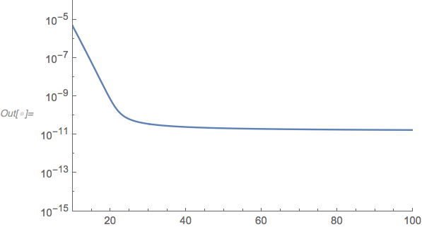
I get thisY vs X plot(Not expected this)

$\endgroup$
4
  • $\begingroup$ Analytical solving seems impossible. $\endgroup$ Commented Apr 23, 2019 at 18:06
  • $\begingroup$ But when i am trying it by giving a boundary condition and suitable range it gives some solutions but it is not even near my expectation $\endgroup$ Commented Apr 23, 2019 at 18:15
  • 1
    $\begingroup$ @DarkKnight45 Example? -- Part of the problem may be the scale of the constants, tho' I think Mariusz is probably right... $\endgroup$
    – Michael E2
    Commented Apr 23, 2019 at 18:48
  • $\begingroup$ @MichaelE2 I have added my scales and also tried to plot it but failed $\endgroup$ Commented Apr 23, 2019 at 20:05

1 Answer 1

5
$\begingroup$

Long comment about the NDSolve example:

The default AccuracyGoal is half working precision or around 8 for MachinePrecision. That means that errors below 10^-8 are treated as acceptable (equivalent to zero). When the value of the solution remains below 10^-8 for a long period, error control basically is turned off, and the solution can bounce around above and below zero. Raising AccuracyGoal can help.

result[x_] = 
  y[x] /. NDSolve[{y'[] == -(2.24794*10^12 ((y[x]^2 - 
              y[x]/10^11 - ((0.000010385 x^3)/E^(2 x)))/x^2)), 
      y[10] == 10^-5.3}, y[x], {x, 10, 100}, 
     AccuracyGoal -> 16][[1]];
LogPlot[result[x], {x, 10, 100}, 
 PlotRange -> {{10, 100}, {10^-15, 10^-4}}]
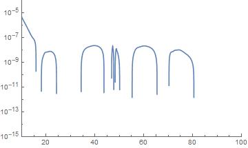
enter image description here

$\endgroup$
5
  • $\begingroup$ Thanks a Lot.You got it correctly $\endgroup$ Commented Apr 24, 2019 at 4:01
  • $\begingroup$ In mathematica changing this accuracy goal slightly changes the results is such randomness permissible in scientific publication $\endgroup$ Commented May 20, 2019 at 5:47
  • $\begingroup$ @DarkKnight45 It should be, but I suppose it depends on what the editors/reviews understand about numerical analysis and Mathematica. With most numerical ODE solvers, each step incurs an error, in which the compute solution steps off the current solution curve onto another that is "near by." How near by depends on the step size. The smaller the step, the smaller the maximum error. As the step size decreases, the "randomness" should go away and the computed solution should converge to a stable result. AccuracyGoal and PrecisionGoal are one way for the user to control the step size. $\endgroup$
    – Michael E2
    Commented May 20, 2019 at 10:56
  • 1
    $\begingroup$ Here's a simple example of how decreasing step size eventually converges toward the exact solution $y = e^{-x}$: Table[ ListLinePlot[ NDSolveValue[{y'[x] + y[x] == 0, y[0] == 1}, y, {x, 0, 60}, Method -> {"FixedStep", Method -> "ExplicitRungeKutta"}, StartingStepSize -> 1.5^k], InterpolationOrder -> 3, PlotLabel -> Row[{"Step size ", 1.5^k}]], {k, 4, -1, -1}] $\endgroup$
    – Michael E2
    Commented May 20, 2019 at 10:59

Your Answer

By clicking “Post Your Answer”, you agree to our terms of service and acknowledge you have read our privacy policy.

Not the answer you're looking for? Browse other questions tagged or ask your own question.