23
$\begingroup$

Lately, we had this thread about interpolation where J. M. linked two interpolation methods. The background for my question is that I estimated a parameter in polar coordinates with dependence on the angle. Therefore, I have a set of values where I know that the values are periodic.

The question is: Is there an easy procedure to interpolate a set of (only a few) points so that the interpolant is monotonic, continuous up to the 1st order derivative, and where the continuous property holds between the start and the end of the interval?

I tried to tweak Interpolation, so if you are interested, please see the following section.

Example and Investigation

Let's define a simple dataset and use Mathematica's Interpolation with PeriodicInterpolation -> True:

data = {{0, 0.2}, {1/3, 0.9}, {2/3, 0.15}, {1, 0.2}};
ip = Interpolation[data, PeriodicInterpolation -> True]
Show[{
      ListLinePlot[data, Mesh -> Full, 
                   MeshStyle -> Directive[Red, PointSize[0.02]]],
      Plot[ip[x], {x, 0, 1}, PlotStyle -> ColorData[1, 2]]
}]
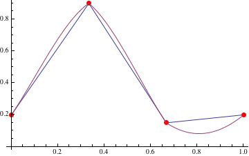
Mathematica graphics

This does not look so bad at a first glance, but the minimum between the last two points violate the monotonicity (which was expected since the interpolation in Mathematica never claimed such a property). Looking at the interpolation graph only and over the interval-boundary shows

Plot[ip[x], {x, 0.2, 1.2}]
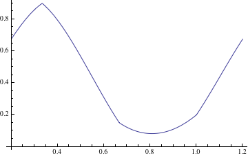
Mathematica graphics

that the derivative is not continuous. Now, my idea was that by using PeriodicInterpolation -> True, I basically tell Mathematica that it can use the values periodically to pad the sides if required. Therefore, a higher interpolation order or maybe using Method -> "Spline" should be able to make the derivatives continuous. When I try to use

Interpolation[data, PeriodicInterpolation -> True, Method -> "Spline"]

I get

Interpolation::mspl: The Spline method could not be used because the data could not be coerced to machine real numbers. >>

which I don't really understand. If I use InterpolationOrder and the default "Hermite" method, I need a value of 20 to get an almost continuous derivative.

Therefore, I tried to do the padding by myself and use "Spline" and a low interpolation order (to reduce the overshooting):

ip2 = Interpolation[
  Join @@ Table[Plus[{i, 0}, #] & /@ Most[data], {i, 0, 10}], 
  InterpolationOrder -> 2, Method -> "Spline"]

Plot[{ip2[x]}, {x, 5, 6.5}, 
     Epilog -> {Red, PointSize[0.02], Point[{5, 0} + # & /@ data]}]
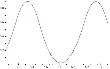
Mathematica graphics

which is of course not monotonic, but at least the derivative is continuous:

Plot[ip2'[x], {x, 5, 6.5}]
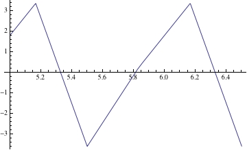
Mathematica graphics

Final solution

I'm accepting the Steffen interpolation in J.M.'s answer as solution for the following reason:

It shows nicely how one can supply derivative values and not only the interpolation values to Interpolation. It therefore does not implement a whole new interpolation but it only calculates adjusted derivatives and uses the internal Interpolation of Mathematica.

Note, that I made some changes in his function. First, the following part

pp = Apply[Dot, Transpose[MapAt[Map[Reverse, #] &,
  Map[Partition[#, 2, 1, {-1, 1}] &, {h, del}], 1]], 1]/
  ListConvolve[{1, 1}, h, {1, -1}];

can be (IMO) slightly simplified to

pp = Dot @@@ Transpose[ MapAt[Reverse, 
  Map[Partition[#, 2, 1, {-1, 1}] &, {h, del}], {1, All}]]/
  ListConvolve[{1, 1}, h, {1, -1}];

which saves a whole pure function and a Map. Otherwise, I combined the periodic and the non-periodic interpolation and added a pattern so that data in the form {y1,y2,...} can be interpolated in the usual way. (Please change the function name. It's only called like that since I included it in a package)

Options[IPCUMonotonicInterpolation] := {
  PeriodicInterpolation -> False
  }

steffenEnds[{{h1_, h2_}, {d1_, d2_}}] := 
 With[{p = d1 + h1 (d1 - d2)/(h1 + h2)}, (Sign[p] + Sign[d1]) Min[
    Abs[p]/2, Abs[d1]]]

IPCUMonotonicInterpolation[data_?(VectorQ[#, NumericQ] &), opts___?OptionQ] :=
    IPCUMonotonicInterpolation[Transpose[{Range[Length[data]], data}], opts];

IPCUMonotonicInterpolation[data_?MatrixQ, OptionsPattern[]] := 
  Module[{dTrans = Transpose[data], del, h, m, pp, optPeriodic, overhangs},
  optPeriodic = OptionValue[PeriodicInterpolation];
  h = Differences[First[dTrans]]; 
  del = Differences[Last[dTrans]]/h;
  overhangs = If[optPeriodic === False, {1, -1}, {-1, 1}];
  (* Note that overhangs in Partition and ListConvolve are defined differently*)
  pp = Dot @@@ Transpose[MapAt[Reverse, 
    Map[Partition[#, 2, 1, overhangs] &, {h, del}], {1, All}]]/
    ListConvolve[{1, 1}, h, -1*overhangs];
  If[optPeriodic === True,
   del = ArrayPad[del, 1, "Periodic"]
   ];
  m = ListConvolve[{1, 1}, 2 UnitStep[del] - 1] *
                MapThread[Min, {Partition[Abs[del], 2, 1], Abs[pp]/2}];
  Interpolation[
   {{#1}, ##2} & @@@ Transpose[Append[dTrans,
      If[optPeriodic === True,
       m,
       Flatten[{
         steffenEnds[#[[{1, 2}]] & /@ {h, del}],
         m,
         steffenEnds[#[[{-1, -2}]] & /@ {h, del}]
         }]
       ]
      ]],
   PeriodicInterpolation -> optPeriodic]
  ]
$\endgroup$
3
  • $\begingroup$ Also relevant: mathematica.stackexchange.com/questions/5929 $\endgroup$
    – s0rce
    Commented Nov 16, 2012 at 3:41
  • $\begingroup$ Your simplification yields somewhat different results from the usual Steffen formula. Witness the difference between Apply[Dot, Transpose[MapAt[Map[Reverse, #] &, Map[Partition[#, 2, 1, {-1, 1}] &, {Table[Subscript[h, k], {k, 5}], Table[Subscript[Δ, k], {k, 5}]}], 1]], 1] and Dot @@@ Transpose[Map[Partition[Reverse[#], 2, 1, {-1, 1}] &, {Table[Subscript[h, k], {k, 5}], Table[Subscript[Δ, k], {k, 5}]}]]. $\endgroup$ Commented Nov 19, 2012 at 11:21
  • $\begingroup$ @J.M. This is hopefully fixed now. $\endgroup$
    – halirutan
    Commented Nov 19, 2012 at 15:36

3 Answers 3

13
$\begingroup$

In fact, halirutan and me already discussed this topic in the chat room only a few days ago, but he thought there should be an explicit question and answer here on main. So, here's my take...

The key here is that the Fritsch-Carlson (the algorithm behind MATLAB's pchip()) and Steffen interpolation methods are both very easily modified to account for periodic data; one only needs to get rid of the special handling of the endpoints, and pad the data accordingly. (A similar treatment can be done for Stineman interpolation, as presented in PlatoManiac's answer, of course.)

Here's the Mathematica implementation for these two $C^1$ interpolation methods:

FritschCarlsonPeriodicInterpolation[data_?MatrixQ] := 
 Module[{dTrans = Transpose[data], del, h, m},
        h = Differences[First[dTrans]]; del = Differences[Last[dTrans]]/h;
        m = If[Equal @@ Sign[Last[#]] && And @@ Thread[Last[#] != 0], 
               3 Total[First[#]]/Total[({{1, 2}, {2, 1}}.First[#])/Last[#]], 0] & /@
            Transpose[{Partition[h, 2, 1, {-1, 1}], Partition[del, 2, 1, {-1, 1}]}];
        Interpolation[MapThread[Append[MapAt[List, #1, 1], #2] &, {data, m}], 
                      PeriodicInterpolation -> True]]

SteffenPeriodicInterpolation[data_?MatrixQ] := 
 Module[{dTrans = Transpose[data], del, h, m, pp},
        h = Differences[First[dTrans]]; del = Differences[Last[dTrans]]/h;
        pp = MapThread[Reverse[#1].#2 &, Map[Partition[#, 2, 1, {-1, 1}] &, {h, del}]]/
             ListConvolve[{1, 1}, h, {1, -1}];
        del = ArrayPad[del, 1, "Periodic"];
        m = ListConvolve[{1, 1}, 2 UnitStep[del] - 1] *
            MapThread[Min, {Partition[Abs[del], 2, 1], Abs[pp]/2}];
        Interpolation[MapThread[Append[MapAt[List, #1, 1], #2] &, {data, m}], 
                      PeriodicInterpolation -> True]]

(Contrast these routines with the implementation of vanilla Fritsch-Carlson here and vanilla Steffen here.)

As an example:

data = {{0, 0.2}, {1/3, 0.9}, {2/3, 0.15}, {1, 0.2}};

ip = Interpolation[data, PeriodicInterpolation -> True];
fcp = FritschCarlsonPeriodicInterpolation[data];
sp = SteffenPeriodicInterpolation[data];

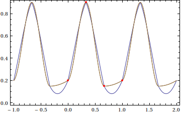
Plot[{ip[t], fcp[t], sp[t]}, {t, -1, 2}, Axes -> None, Frame -> True, 
     Epilog -> {Directive[AbsolutePointSize[4], Red], Point[data]}]

shape-preserving periodic interpolants

The Steffen and Fritsch-Carlson periodic interpolants are nigh-indistinguishable, but do a better job of preserving the shape of the data than the default periodic interpolation method.

$\endgroup$
15
$\begingroup$

One can look at the paper here. However, from the Wolfram Library Archive, I got this ready-made code that needed only the CompilationTarget -> "C" part to modernize:

StinemanInterpolatingFunction::dmval=
"Input value lies outside domain of the interpolating function.";
Format[StinemanInterpolatingFunction[range_,_]]:=
SequenceForm["StinemanInterpolatingFunction[",range,", <>]"];
lin=Compile[{x0,y0,x1,y1,x},(y0(x1-x)+y1(x-x0))/(x1-x0),
CompilationTarget-> "C"];
delta=Compile[{x0,y0,y0p,x,linint},(y0+y0p (x-x0)-linint),
CompilationTarget-> "C"];
sC=Compile[{x0,x1,x,linint,delta0,delta1},
linint+delta0*delta1*
If[delta0*delta1>0,
1/(delta0+delta1),
If[delta0*delta1==0,
    0,
    (2x-x0-x1)/((delta0-delta1)(x1-x0))
    ]
    ],
CompilationTarget-> "C"];
home[{_,_},_]:=1;
home[xvals_,x_]:=Module[{n=Length[xvals],h},
h=Quotient[n,2];
Which[x<xvals[[h]],
home[Take[xvals,h],x],x>xvals[[h+1]],h+home[Take[xvals,h-n],x],True,h]
];
endslope[{x1_,y1_},{x2_,y2_},s2_]:=Module[{z=(y2-y1)/(x2-x1)},
z+If[!Negative[z (z-s2)],
z-s2,
1/(1/(z-s2)+Sign[z-s2]/Abs[z])]
];
augment[data_]:=Module[{temp1,temp2,dTrans,yji,ykj,xji,xkj,midslopes},
dTrans=Transpose[data];
{xji,yji}=Rest[Drop[#,-1]]-Drop[#,-2]&/@dTrans;
{xkj,ykj}=Drop[#,2]-Rest[Drop[#,-1]]&/@dTrans;
{temp1,temp2}={xkj^2+ykj^2,xji^2+yji^2};
midslopes=(yji temp1+ykj temp2)/(xji temp1+xkj temp2);
Transpose[{data,Join[{endslope[First[data],data[[2]],First[midslopes]]},midslopes,
                {endslope[Last[data],data[[-2]],Last[midslopes]]}]}]
];
StinemanInterpolation[data_]:=
StinemanInterpolatingFunction[data[[{1,-1},1]],augment[N[data]]];
StinemanInterpolatingFunction[{r_,s_},data_][x_?NumberQ]:=
Message[StinemanInterpolatingFunction::dmval]/;!(r<=x<=s);
StinemanInterpolatingFunction[{r_,s_},adata_][x_?NumberQ]:=
Module[{d,linearInt},
d=Flatten[{adata[[home[First/@First[Transpose[adata]],x]+{0,1}]],x}];
Apply[sC,Join[d[[{1,4,7}]],
     {linearInt=lin@@d[[{1,2,4,5,7}]],
     delta@@Join[d[[{1,2,3}]],{x,linearInt}],delta@@Join[d[[{4,5,6}]],
     {x,linearInt}]}]]
];

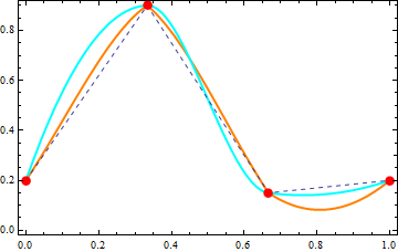
Now this seems to work well:

data = {{0, 0.2}, {1/3, 0.9}, {2/3, 0.15}, {1, 0.2}};
ip = Interpolation[data, PeriodicInterpolation -> True];
f1 = StinemanInterpolation[data];
Show[{Plot[Evaluate[{ip[x], f1[x]}], {x, 0, 1}, 
     PlotStyle -> {{Thick, Orange}, {Thick, Cyan}}], 
     ListLinePlot[data, Mesh -> Full, PlotStyle -> Dashed, 
     PlotRange -> All, MeshStyle -> Directive[Red, PointSize[0.025]]]}, 
   Frame -> True, Axes -> False]

plot of interpolant

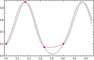
The padded data also works as expected:

ip2=Interpolation[Join@@Table[Plus[{i,0},#]&/@Most[data],{i,0,10}],
      InterpolationOrder->2,Method->"Spline"];
f2=StinemanInterpolation[Join@@Table[Plus[{i,0},#]&/@Most[data],{i,0,10}]];
Plot[{ip2[x],f2[x]},{x,5,6.5},
   Epilog->{Red,PointSize[0.02],Point[{5,0}+#&/@data]},
   Frame-> True,Axes-> False,PlotRange-> All]

plot of interpolant of padded data

BR

$\endgroup$
8
  • $\begingroup$ Thanks for sharing this. It looks like the JSTOR paper you are linking to discusses 2D interpolation. Did you mean some other reference? $\endgroup$
    – Sasha
    Commented Nov 15, 2012 at 16:47
  • $\begingroup$ Wikipedia provides more relevant references in the article on monotone cubic interpolation. $\endgroup$
    – Sasha
    Commented Nov 15, 2012 at 16:52
  • 1
    $\begingroup$ @Sasha, yes, the method in that paper Plato linked to is for bivariate interpolation. Probably he intended to link to this (and I gave implementations here). $\endgroup$ Commented Nov 15, 2012 at 16:52
  • $\begingroup$ Nice one (+1)... $\endgroup$
    – halirutan
    Commented Nov 15, 2012 at 16:56
  • $\begingroup$ @hal, the Stineman scheme can certainly be readapted for periodic data (e.g. remove the endslope[] bits, as well as modifying the interval bisection routine home[])... $\endgroup$ Commented Nov 15, 2012 at 16:58
10
$\begingroup$

Being rather dissatisfied with the implementation of Stineman interpolation presented here (among other things, the computation of endslope[] is superfluous, as previously noted), I decided to roll out my own implementation of periodized Stineman interpolation. Here it is:

StinemanPeriodicSlopes[data_?MatrixQ] := With[{sq = {#2.#2, #1.#1}},
        {#1[[2]], #2[[2]]}.sq/{#1[[1]], #2[[1]]}.sq] & @@@
        Partition[Differences[data], 2, 1, {-1, 1}]

StinemanPeriodicInterpolation::inddp = "The point `1` is duplicated.";

StinemanPeriodicInterpolation[data_] := Module[{diffs, times},
  StinemanInterpolatingFunction[data[[{1, -1}, 1]], 
          Append[Transpose[data], StinemanPeriodicSlopes[data]], True] /; 
          If[MemberQ[diffs = Chop[Differences[times = data[[All, 1]]]], 0], 
             Message[StinemanPeriodicInterpolation::inddp, 
                     First[Extract[times, Position[diffs, 0]]]]; False, True]]

StinemanInterpolatingFunction::dmval =
     "Input value `1` lies outside the domain of the interpolating function.";

Format[StinemanInterpolatingFunction[range_, __]] := 
       SequenceForm["StinemanInterpolatingFunction[", range, ", <>]"]

StinemanInterpolatingFunction[{p_, q_}, data_, False][x_?NumericQ] :=
     (Message[StinemanInterpolatingFunction::dmval, x]; $Failed) /; ! (p <= x <= q)

StinemanInterpolatingFunction[{p_, q_}, data_, perQ_][x_?NumericQ] := 
     Module[{dl, dp, dr, h, l, li, m, r, t, tl, tr, xa, ya, yp},
            {xa, ya, yp} = data;

            t = If[perQ, Mod[x, q - p, p], x];

            l = 1; r = Length[xa];
            While[r - l > 1,
                  m = Quotient[l + r, 2];
                  If[t < xa[[m]], r = m, l = m]];

            tl = t - xa[[l]]; tr = t - xa[[r]]; h = xa[[r]] - xa[[l]];
            li = {-ya[[l]], ya[[r]]}.{tr, tl}/h;
            dl = ya[[l]] + yp[[l]] tl - li; dr = ya[[r]] + yp[[r]] tr - li;
            dp = dl dr;
            li + dp Switch[Sign[dp], 1, 1/(dl + dr), 0, 0, -1, (tl + tr)/(h (dl - dr))]]

For comparison purposes, here's how to use Stineman's slope formula with Hermite interpolation:

StinemanHermitePeriodicInterpolation[data_] := Interpolation[
  MapThread[Append[MapAt[List, #1, 1], #2] &,
            {data, StinemanPeriodicSlopes[data]}], PeriodicInterpolation -> True]

Here's OP's data set, again:

data = {{0, 0.2}, {1/3, 0.9}, {2/3, 0.15}, {1, 0.2}};

Here's two periodic interpolants:

st = StinemanPeriodicInterpolation[data];
sh = StinemanHermitePeriodicInterpolation[data];

Plot 'em:

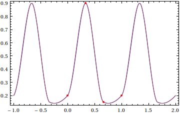
Plot[{st[t], sh[t]}, {t, -1, 2}, Axes -> None, Frame -> True, 
     Epilog -> {Directive[AbsolutePointSize[4], Red], Point[data]}]

periodized Stineman interpolants

I've already made provisions for the possibility of combining the periodic and nonperiodic versions of Stineman interpolation, but I'll leave the actual implementation as an exercise for the involved reader.

$\endgroup$

Your Answer

By clicking “Post Your Answer”, you agree to our terms of service and acknowledge you have read our privacy policy.

Not the answer you're looking for? Browse other questions tagged or ask your own question.