85
$\begingroup$

Stan Wagon's Mathematica in Action (second edition; I haven't read the third edition and I'm hoping to eventually see it), demonstrates a nifty function called FindAllCrossings2D[]. What the function basically does is to augment FindRoot[] by using ContourPlot[] to find crossings that FindRoot[] can subsequently polish. Here, Wagon uses the function to assist in solving one of the questions of the SIAM hundred-digit challenge.

ContourPlot[] changed quite a bit starting from version 6 (e.g., it now outputs GraphicsComplex[] objects), and FilterRules[] has superseded the old standby FilterOptions[] With these in mind, I set out to update FindAllCrossings2D[]:

Options[FindAllCrossings2D] = 
  Sort[Join[Options[FindRoot], {MaxRecursion -> Automatic, 
     PerformanceGoal :> $PerformanceGoal, PlotPoints -> Automatic}]];

FindAllCrossings2D[funcs_, {x_, xmin_, xmax_}, {y_, ymin_, ymax_}, opts___] := 
 Module[{contourData, seeds, tt, fy = Compile[{x, y}, Evaluate[funcs[[2]]]]},

  contourData = Map[First, Cases[
     Normal[
      ContourPlot[funcs[[1]], {x, xmin, xmax}, {y, ymin, ymax},
       Contours -> {0}, ContourShading -> False, 
       PlotRange -> {Full, Full, Automatic}, 
       Evaluate[
        Sequence @@ 
         FilterRules[Join[{opts}, Options[FindAllCrossings2D]], 
          DeleteCases[Options[ContourPlot], Method -> _]]]
       ]], _Line, Infinity]];

  seeds = Flatten[Map[#[[
       1 + Flatten[Position[Rest[tt = Sign[Apply[fy, #, 2]]] Most[tt], -1]]
                ]] &, contourData], 1];

  If[seeds == {}, seeds,
   Select[
    Union[Map[{x, y} /. 
        FindRoot[{funcs[[1]] == 0, 
          funcs[[2]] == 0}, {x, #[[1]]}, {y, #[[2]]}, 
         Evaluate[
          Sequence @@ 
           FilterRules[Join[{opts}, Options[FindAllCrossings2D]], 
            Options[FindRoot]]]] &, 
      seeds]], (xmin < #[[1]] < xmax && ymin < #[[2]] < ymax) &]]]

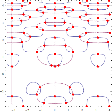
The function works splendidly, it seems. I tried out the same example Wagon used in his book:

f[x_, y_] := -Cos[y] + 2 y Cos[y^2] Cos[2 x];
g[x_, y_] := -Sin[x] + 2 Sin[y^2] Sin[2 x];

pts = FindAllCrossings2D[{f[x, y], g[x, y]}, {x, -7/2, 4}, {y, -9/5, 21/5},
                         Method -> {"Newton", "StepControl" -> "LineSearch"}, 
                         PlotPoints -> 85, WorkingPrecision -> 20] // Chop;

ContourPlot[{f[x, y], g[x, y]}, {x, -7/2, 4}, {y, -9/5, 21/5},
        Contours -> {0}, ContourShading -> False, 
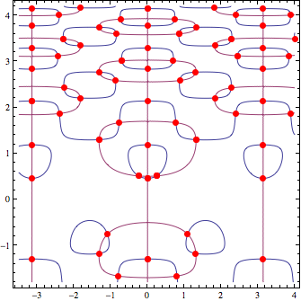
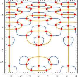
        Epilog -> {AbsolutePointSize[6], Red, Point /@ pts}]

FindAllCrossings2D[] example

Whew, that preamble was quite long. Here's my question, then:

Are there "neater" (for some definition of "neater") ways to update/reimplement FindAllCrossings2D[] than my attempt?

$\endgroup$
5
  • 1
    $\begingroup$ Could someone come up with a Google Books link that works in Europe? $\endgroup$
    – Szabolcs
    Commented Jan 20, 2012 at 13:04
  • $\begingroup$ @Szabolcs What about this here books.google.de/… $\endgroup$
    – halirutan
    Commented Jan 25, 2012 at 2:29
  • 2
    $\begingroup$ As a tiny note: one unexpected benefit of the ContourPlot[] approach is that one can exploit the RegionFunction option if one is only interested in roots within a given region. $\endgroup$ Commented Jan 25, 2012 at 10:35
  • $\begingroup$ @J.M. I just posted a new version using ContourPlot[] - seems very short. $\endgroup$ Commented Jan 26, 2012 at 6:08
  • $\begingroup$ I noticed, @Vitaliy; sadly I can't upvote again... $\endgroup$ Commented Jan 26, 2012 at 6:09

9 Answers 9

57
$\begingroup$

Here is my latest code for this function, from Chapter 12 of the third edition of "Mathematica in Action". It is pretty short, but I will let you work out if it is faster or more robust than yours. Note the PlotPoints option for difficult cases.

FindRoots2D::usage = 
  "FindRoots2D[funcs,{x,a,b},{y,c,d}] finds all nontangential solutions to
   {f=0, g=0} in the given rectangle."; 

Options[FindRoots2D] = {PlotPoints -> Automatic, MaxRecursion -> Automatic}; 

FindRoots2D[funcs_, {x_, a_, b_}, {y_, c_, d_}, opts___] := Module[
  {fZero, seeds, signs, fy}, 
  fy = Compile[{x, y}, Evaluate[funcs[[2]]]]; 

  fZero = Cases[Normal[
     ContourPlot[
        funcs[[1]] == 0, 
        {x, a-(b-a)/97, b+(b-a)/103}, {y, c-(d-c)/98, d+(d-c)/102}, 
        Evaluate[FilterRules[{opts}, Options[ContourPlot]]]]], 
     Line[z_] :> z, Infinity]; 

  seeds = Flatten[(
     (signs = Sign[Apply[fy, #1, {1}]]; 
      #1[[1 + Flatten[Position[Rest[signs*RotateRight[signs]], -1]]]]) &
     ) /@ fZero, 1];
  If[seeds == {}, {}, 
     Select[
        Union[({x, y} /.
           FindRoot[{funcs[[1]], funcs[[2]]}, {x, #1[[1]]}, {y, #1[[2]]}, 
              Evaluate[FilterRules[{opts}, Options[FindRoot]]]] & ) /@ seeds, 
           SameTest -> (Norm[#1 - #2] < 10^(-6) & )], 
        a <= #1[[1]] <= b && c <= #1[[2]] <= d & ]]]
$\endgroup$
7
  • $\begingroup$ Hi Dr. Wagon! Thanks for posting your updated code (and for the book in general; I hope I can get a copy of your new one some day); I'll do the tests later for this! I've also found that RegionFunction can be profitably used here to restrict the search to roots within a domain. $\endgroup$ Commented Jan 26, 2012 at 4:36
  • 4
    $\begingroup$ BTW: is there anything special about the increments chosen in {x, a-(b-a)/97, b+(b-a)/103}, {y, c-(d-c)/98, d+(d-c)/102}? $\endgroup$ Commented Jan 26, 2012 at 5:36
  • 1
    $\begingroup$ Oh. Would you happen to have a set of equations on hand where the asymmetry in ContourPlot[] is a necessity? $\endgroup$ Commented Jan 26, 2012 at 23:09
  • 2
    $\begingroup$ Not on hand. But this function is used many many times in the VisualDSolve project to find equilibrium points for two autonomous DEs and I must have found some difficult examples there. Now, it is possible as Mathematica changes internally that some of the problems disappear. Let me mention that this function was able to solve one of the "100 Digit Challenge" problems in optimizing a complicated function of 2 vbles by finding all of the critical points in the region, and there were well over 2000 of them. $\endgroup$
    – stan wagon
    Commented Jan 27, 2012 at 15:21
  • 4
    $\begingroup$ There is a small problem with how the Compile arguments are being handled here. With the setting SetSystemOptions["StrictLexicalScoping" -> True]; this function fails due to x and y being renamed in Compile[{x,y}, ...] but not in funcs. $\endgroup$
    – Szabolcs
    Commented Aug 8, 2016 at 11:42
38
$\begingroup$

This is ContourPlot based but seems much shorter:

FindCrossings2D[{f_, g_}, {x_, xmin_, xmax_}, {y_, ymin_, ymax_}] := 
  {x, y} /. (FindRoot[{f[x, y] == 0, g[x, y] == 0}, {{x, #[[1]]}, 
  {y, #[[2]]}}] & /@ (ContourPlot[{f[x, y] == 0, g[x, y] == 0}, 
  {x, xmin, xmax}, {y, ymin, ymax}][[1, 1]]))

It works:

f[x_, y_] := -Cos[y] + 2 y Cos[y^2] Cos[2 x];
g[x_, y_] := -Sin[x] + 2 Sin[y^2] Sin[2 x];

pts = FindCrossings2D[{f, g}, {x, -7/2, 4}, {y, -9/5, 21/5}];

ContourPlot[{f[x, y] == 0, g[x, y] == 0}, {x, -7/2, 4}, {y, -9/5, 
  21/5}, Epilog -> {AbsolutePointSize[6], Red, Point /@ pts}]

enter image description here

$\endgroup$
1
  • $\begingroup$ Nice work! I'm amazed by so short codes. $\endgroup$
    – yulinlinyu
    Commented May 17, 2012 at 14:27
35
$\begingroup$

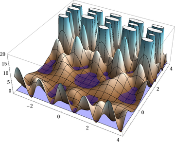
Let me give a different approach. FindRoot does a good job, but maybe we can calculate the seed-points in a different way. When you want to find the common roots of $f(x,y)$ and $g(x,y)$ you can transform the problem into one equation which has the same roots $$0=f(x,y)^2+g(x,y)^2$$ The nice property here, which I will use is that the right hand side of this equation is always greater than zero. The bad thing is, that functions that don't cross zero are kind of difficult for some numerical methods, but that will be no concern here.

When we look at our function and think of it as a kind of water-pool with a very low level of water, you would get something like this

enter image description here

Now the idea is to go around each of those small pools which have maybe one, maybe more local zeroes in it, and start from every coast point a root-search.

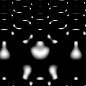
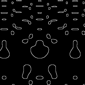
That's the time where the image-processing kicks in. Our function is always positive which gives a really nice image (I inverted gray-levels):

enter image description here

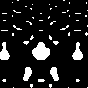
Cutting off the image at sea-level is just a binarization of the image.

enter image description here

Finding the coast-line of each pool is simply implemented by an image subtraction and a dilation of the binarized image.

enter image description here

The complete method is therefore to raster the above function, extract all coast-pixel with image processing and run FindRoot for each coast-point.

FindCrossings2D[{f_, g_}, {x_, xmin_, xmax_}, {y_, ymin_, ymax_}, 
                 n_, threshold_] := Module[
{seeds = ImageData[ImageSubtract[Dilation[#, 1], #] &@
  Binarize[ColorNegate[Image[
         Table[f[x, y]^2 + g[x, y]^2, 
          {y, ymin, ymax, (ymax - ymin)/(n - 1.0)}, 
          {x, xmin, xmax, (xmax - xmin)/(n - 1.0)}]]], 
       threshold], "Bit"]},
  DeleteDuplicates[Last@Last@Reap[MapIndexed[
    If[#1 === 1, Sow[{x, y} /. FindRoot[{f[x, y] == 0, g[x, y] == 0}, 
     {{x, Rescale[#2[[2]], {1, n}, {xmin, xmax}]},
      {y, Rescale[#2[[1]], {1, n}, {ymin, ymax}]}}]]] &, seeds, 2]
   ], (Norm[#1 - #2] < 10.^(-6)) &]
] 

Here n is the raster-size and thresh is the binarization threshold which should be a bit smaller than 1.

f[x_, y_] := -Cos[y] + 2 y Cos[y^2] Cos[2 x];
g[x_, y_] := -Sin[x] + 2 Sin[y^2] Sin[2 x];

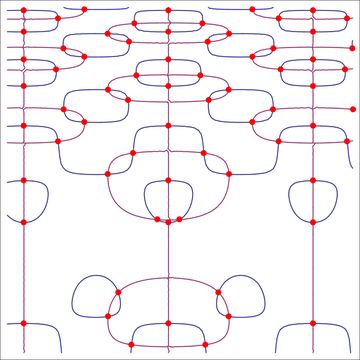
roots = FindCrossings2D[{f, g}, {x, -7/2, 4}, {y, -9/5, 21/5}, 400, 0.8];

enter image description here

This approach has clearly the disadvantage of having a fixed raster size, while ContourPlot uses adaptive sampling. Nevertheless, for raster-sizes from 200-500 and thresholds from ?-0.95 the method finds all or at least many roots.

$\endgroup$
2
  • 1
    $\begingroup$ Interesting approach. When I tried FindCrossings2D[{f, g}, {x, -7/2, 4}, {y, -9/5, 21/5}, 400, 0.8] on my system, it only got 59 out of the 67 roots within the region. (Increasing the value of the fourth argument gradually eventually yielded the roots, but takes quite a bit of time to execute.) I guess choosing appropriate parameters can be system-dependent... $\endgroup$ Commented Jan 25, 2012 at 10:22
  • 3
    $\begingroup$ For the record, the new-in-8 functions ContourDetect (and CrossingDetect) would come handy with this approach. $\endgroup$ Commented Jan 27, 2012 at 13:02
25
$\begingroup$

You could use MorphologicalBranchPoints in combination with ContourPlot to find the seeds for the intersection points. Consider for example

f[x_, y_] := -Cos[y] + 2 y Cos[y^2] Cos[2 x];
g[x_, y_] := -Sin[x] + 2 Sin[y^2] Sin[2 x];

range = {{-7/2, 4}, {-9/5, 21/5}};

First we create a binarized, thinned image of the contour plot.

binPlot = Thinning@Binarize[Image[ContourPlot[{f[x, y], g[x, y]},
   {x, range[[1, 1]], range[[1, 2]]},
   {y, range[[2, 1]], range[[2, 2]]},
   Contours -> {0}, PlotPoints -> 30,
   ContourStyle -> White, Background -> Black, 
   PlotRangePadding -> 0, Frame -> False]]];

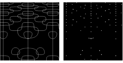
After applying MorphologicalBranchPoints on this image we find

intersPlot = MorphologicalBranchPoints[binPlot];
GraphicsGrid[{{binPlot, Dilation[intersPlot, 1]}}]

Mathematica graphics

Then the seeds are just the rescaled positions of 1 in the ImageData of intersPlot.

seeds = DeleteDuplicates[
  Position[Reverse[ImageData[intersPlot]], 2].{{0, 1}, {1, 0}}, 
  (ChessboardDistance[#1, #2] <= 1) &];
seeds = Transpose[N@MapThread[
   Rescale[#, {1, #2}, #3] &, 
   {Transpose[seeds], ImageDimensions[intersPlot], range}, 1]];

The intersection points can then be found using FindRoot as before

crossp = {x, y} /. Quiet@FindRoot[{f[x, y] == 0, g[x, y] == 0}, 
  {x, #1}, {y, #2}] & @@@ seeds;
DeleteDuplicates[crossp, (Norm[#1 - #2] < .0001 &)]

Show[ContourPlot[{f[x, y], g[x, y]}, {x, -7/2, 4}, {y, -9/5, 21/5}, 
    Contours -> {0}, PlotPoints -> 30],
  Graphics[{PointSize[Large], Red, Point[crossp]}]
]

Mathematica graphics

$\endgroup$
22
$\begingroup$

This method is based on the MeshFunctions. Detailed description is in this post:

Clear[f, g]
f[x_, y_] := -Cos[y] + 2 y Cos[y^2] Cos[2 x];
g[x_, y_] := -Sin[x] + 2 Sin[y^2] Sin[2 x];

Show[{
        ContourPlot[{f[x, y] == 0, g[x, y] == 0},
            {x, -7/2, 4}, {y, -9/5, 21/5},
            ContourStyle -> {Lighter[Brown, .7], GrayLevel[.7]}],
        ContourPlot[f[x, y] == 0,
            {x, -7/2, 4}, {y, -9/5, 21/5},
            ContourStyle -> None,
            MeshFunctions -> Function[{x, y, z}, g[x, y]],
            Mesh -> {{0}},
            MeshStyle -> Directive[Red, AbsolutePointSize[4]]
            ]
        }]

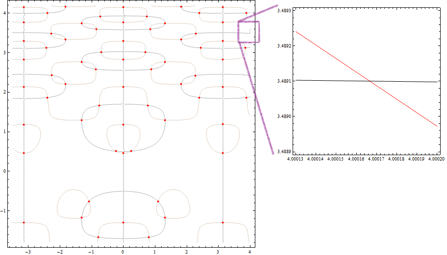
all cross points in the range

Note the amplified area, the cross point there is actually out of the specified range. Expanding the x range and using option PlotPoints -> 300, we can obtain this point:

Show[{
        ContourPlot[{f[x, y] == 0, g[x, y] == 0},
            {x, -7/2, 4.0002}, {y, -9/5, 21/5},
            ContourStyle -> {Lighter[Brown, .7], GrayLevel[.7]}],
        ContourPlot[f[x, y] == 0,
            {x, -7/2, 4.0002}, {y, -9/5, 21/5},
            PlotPoints -> 300,
            ContourStyle -> None,
            MeshFunctions -> Function[{x, y, z}, g[x, y]],
            Mesh -> {{0}},
            MeshStyle -> Directive[Red, AbsolutePointSize[4]]
            ]
        }]
$\endgroup$
4
  • $\begingroup$ This is very nice (+1)! A side-question: what do you use for the zoomed area? Is it within Mathematica or externally? $\endgroup$
    – gpap
    Commented Apr 22, 2014 at 14:07
  • $\begingroup$ @gpap Thanks. It's the crayon style in the Paint in Windows 8 :) But I believe it can be implemented in MMA. $\endgroup$
    – Silvia
    Commented Apr 22, 2014 at 14:09
  • $\begingroup$ Couldn't this be even simpler by using ContourPlot[{f[x, y] == 0, g[x, y] == 0}, {x, -7/2, 4}, {y, -9/5, 21/5}, MeshFunctions -> {f[#1, #2] - g[#1, #2] &}, Mesh -> {{0}}, MeshStyle -> Directive[Red, PointSize[Large]]]? $\endgroup$
    – Jason B.
    Commented Aug 18, 2016 at 17:29
  • $\begingroup$ @JasonB My first ContourPlot is for visualization only, which is unnecessary if one just wants to find the crossing. The second ContourPlot is for solving the equation. Including only one of f[x,y]==0 and g[x,y]==0 as the target in it will notably reduce the computing time. $\endgroup$
    – Silvia
    Commented Aug 20, 2016 at 13:28
19
$\begingroup$

Here is my revision of Stan Wagon's 3rd Edition function.

It is again faster and IMHO cleaner.

FindRoots2D::usage = 
  "FindRoots2D[funcs,{x,a,b},{y,c,d}] finds all nontangential solutions to
   {f=0, g=0} in the given rectangle."; 

Options[FindRoots2D] = {PlotPoints -> Automatic, 
   MaxRecursion -> Automatic};

FindRoots2D[
  funcs : {f1_, f2_}, {x_, a_, b_}, {y_, c_, d_}, opts : OptionsPattern[]
] :=
 Module[{fZero, seeds, fy = Compile[{x, y}, f2]},

  fZero =
    Cases[
      Normal @ ContourPlot[
        f1 == 0,
        {x, a - (b-a)/97, b + (b-a)/103},
        {y, c - (d-c)/98, d + (d-c)/102},
        Evaluate @ FilterRules[{opts}, Options @ ContourPlot] ],
      Line[z_] :> z,
      Infinity
   ];

  seeds = 
    Pick[Rest@#, Rest[#]Most[#]& @ Sign @ Apply[fy, #, 2], -1] & /@ fZero;

  With[{seq = FilterRules[{opts}, Options @ FindRoot]},
    Select[
      Union[
        {x, y} /. FindRoot[funcs, {x, #}, {y, #2}, seq] & @@@ Join @@ seeds,
        SameTest -> (Norm[# - #2] < 1*^-6 &)],
      a <= #[[1]] <= b && c <= #[[2]] <= d &] ]
 ]
$\endgroup$
16
$\begingroup$

Here's a way that's somewhat more efficient than FindRoots2D. I use Plot3D instead of ContourPlot, but more importantly for speed, I use ListPlot to approximate the zeros of the second function along the first. These are then polished with FindRoot as in other answers.

ClearAll[findAllRoots2D];
Options[findAllRoots2D] = Join[Options[FindRoot], Options[Plot3D]];

findAllRoots2D[{f1_, f2_}, {x_, a_, b_}, {y_, c_, d_}, opts___] :=
 Module[{f1plot, f2plot},
  f1plot = Plot3D[f1, {x, a, b}, {y, c, d},
    MeshFunctions -> {Function @@ {{x, y}, f1}},
    Mesh -> {{0}}, PlotStyle -> None,
    PlotRange -> All, BoundaryStyle -> None, Method -> Automatic,
    Evaluate@FilterRules[{opts}, Options[Plot3D]]];
  f2plot = ListLinePlot[
    Cases[Normal@f1plot, Line[pts_] :> pts[[All, {1, 2}]], Infinity],
    MeshFunctions -> {Function @@ {{x, y}, f2}},
    Mesh -> {{0}}
    ];
  Quiet[Check[
      FindRoot[{f1 == 0, f2 == 0}, {x, #[[1]], a, b}, {y, #[[2]], c, d},
        Evaluate@FilterRules[{opts}, Options[FindRoot]]], 
      Unevaluated@Sequence[], FindRoot::reged], FindRoot::reged] & /@ 
   Cases[Normal@f2plot, Point[p_] :> p, Infinity]
  ];

On the example:

f[x_, y_] := -Cos[y] + 2 y Cos[y^2] Cos[2 x];
g[x_, y_] := -Sin[x] + 2 Sin[y^2] Sin[2 x];

pts = {x, y} /. 
    findAllRoots2D[{f[x, y], g[x, y]}, {x, -7/2, 4}, {y, -9/5, 21/5}, 
     Method -> {"Newton", "StepControl" -> "LineSearch"}, 
     PlotPoints -> 85, WorkingPrecision -> 20]; // AbsoluteTiming
(*  {11.8102, Null}  *)

ContourPlot[{f[x, y], g[x, y]}, {x, -7/2, 4}, {y, -9/5, 21/5}, 
 Contours -> {0}, ContourShading -> False, 
 Epilog -> {AbsolutePointSize[6], Red, Point@pts}]

Mathematica graphics

FindRoots2D takes about 7 seconds longer:

FindRoots2D[{f[x, y], g[x, y]}, {x, -7/2, 4}, {y, -9/5, 21/5},
     Method -> {"Newton", "StepControl" -> "LineSearch"}, 
    PlotPoints -> 85, WorkingPrecision -> 20]; // AbsoluteTiming
(*  {18.6097, Null}  *)

Mr. Wizard's improvement was 1 sec. faster than FindRoots2D.

$\endgroup$
4
  • $\begingroup$ It's probably best to stick Method -> Automatic somewhere in the options for f1plot so that Method options for FindRoot[] cannot interfere with the plotting in any way. Now that I think about it, the speed may be due to the fact that Plot3D[] does a coarser mesh sampling than ContourPlot[]. $\endgroup$ Commented Oct 27, 2015 at 1:04
  • $\begingroup$ @J.M. Thanks for the suggestion. The mesh lines have 1200 more points than the contour lines (for f1). Of course, accuracy also has to do with how the adaptive sampling is carried out. 1200 more points in useless locations don't really help. But Plot3D runs 4-5 sec. faster than ContourPlot. $\endgroup$
    – Michael E2
    Commented Oct 27, 2015 at 1:27
  • $\begingroup$ Really... my experience with MeshFunctions is that they often give slightly rougher-looking lines than ContourPlot[]'s. Oh well, I guess another one of Mathematica's mysteries. $\endgroup$ Commented Oct 27, 2015 at 1:34
  • $\begingroup$ @J.M. Maybe it's the PlotPoints -> 85 in the example. Perhaps with defaults, ContourPlot usually does better. $\endgroup$
    – Michael E2
    Commented Oct 27, 2015 at 1:41
15
$\begingroup$

Here is your own code cleaned up a bit. It runs about a third faster and most of the time is spent on ContourPlot.

Options[FindAllCrossings2D] = 
  Sort[Join[Options[FindRoot], {MaxRecursion -> Automatic, 
     PerformanceGoal :> $PerformanceGoal, PlotPoints -> Automatic}]];

FindAllCrossings2D[
 {func1_, func2_},
 {x_, xmin_, xmax_},
 {y_, ymin_, ymax_},
 opts___
] :=
 Module[{contourData, seeds, optsflt, fy = Compile[{x, y}, func2]},

  optsflt[fname_] := Sequence @@
    FilterRules[{opts} ~Join~ Options@FindAllCrossings2D, Options@fname];

  contourData =
    Cases[ Normal @ ContourPlot[
       func1, {x, xmin, xmax}, {y, ymin, ymax}, Contours -> {0}, 
       ContourShading -> False, PlotRange -> {Full, Full, Automatic}, 
       Method -> Automatic, Evaluate[optsflt @ ContourPlot] ],
     L_Line :> L[[1]],
     Infinity
    ];

  seeds = 
    Pick[Rest@#, Rest[#]Most[#]& @ Sign @ Apply[fy, #, 2], -1] & /@ contourData;

  Select[
   Union @ With[{seq = optsflt @ FindRoot},
     {x, y} /. FindRoot[{func1 == 0, func2 == 0}, {x, #1}, {y, #2}, seq] &
       @@@ Join @@ seeds],
   (xmin < #[[1]] < xmax && ymin < #[[2]] < ymax) &]

 ]
$\endgroup$
13
$\begingroup$

I am not sure if it is worth pointing out (it might even be mentioned in Stan Wagon’s book - I have the second edition, but as I am away from home I can’t check it) that these particular system of equations can be solved by Mathematica (or, more precisely with the help of Mathematica) exactly (by means of Reduce) so that all these initial points etc., are quite unnecessary. Here is how you do it:

eq1 = TrigExpand[g[x, y]];

eq2 = TrigExpand[f[x, y]] /. Sin[x]^2 -> 1 - Cos[x]^2;

eq = Eliminate[{eq1 == 0, eq2 == 0}, Cos[x]];

solsNonzero = Reduce[Sin[x] != 0 && eq && -5 <= y <= 5, y];

solsZero = Reduce[Sin[x] == 0 && eq && -5 <= y <= 5, y];

sols1 = {x, y} /. 
   N[{ToRules[
      Reduce[solsNonzero && 
        eq1 == 0 && -5 <= x <= 5 && -5 <= y <= 5, {y, x}]]}];

sols2 = {x, y} /. 
   N[{ToRules[
      Reduce[solsZero && f[x, y] == 0 && 
        g[x, y] == 0 && -5 <= x <= 5 && -5 <= y <= 5, {y, x}]]}];

sols = Join[sols1, sols2];

ContourPlot[{f[x, y], g[x, y]}, {x, -5, 5}, {y, -5, 5}, 
 Contours -> {0}, ContourShading -> False, 
 Epilog -> {AbsolutePointSize[6], Red, Point /@ sols}]

If you evaluate all the above you should see the already all too familiar picture.

$\endgroup$
1
  • $\begingroup$ Sure; I was just looking for a test function for FindAllCrossings2D[] and I used Stan Wagon's example. I however use it for more complicated transcendental equations, and the proper analysis is just a liiitle bit out of reach... but thanks for giving the analytical solution. $\endgroup$ Commented Jan 26, 2012 at 16:54

Your Answer

By clicking “Post Your Answer”, you agree to our terms of service and acknowledge you have read our privacy policy.

Not the answer you're looking for? Browse other questions tagged or ask your own question.