Interpolating an Antiderivative

Question

I'd like to be able to make InterpolatingFunctions for antiderivatives of functions that can't be integrated symbolically. However, the following code returns several error messages:

FunctionInterpolation[Integrate[Sqrt[1 + x^3], {x, 0, t}], {t, 0, 10}]

Here are the messages:

Thread::tdlen: "Objects of unequal length in {-1.25,-0.416667,0.416667,1.25}^{} cannot be combined. "

Thread::tdlen: "Objects of unequal length in {0.223144 +3.14159\ I,-0.875469+3.14159\ I,-0.875469,0.223144}\ {}\n cannot be combined. "

Thread::tdlen: "Objects of unequal length in {-1.25,-0.416667,0.416667,1.25}\ {} cannot be combined."

General::stop: "Further output of Thread::tlden will be suppressed during this calculation."

FunctionInterpolation::nreal: Near t = 1.25`, the function did not evaluate to a real number.

FunctionInterpolation::nreal: Near t = 1.3277777777777777`, the function did not evaluate to a real number.

What's going on? Is there a simple way to make this work? Changing Integrate to NIntegrate doesn't help, though the error messages are different:

NIntegrate::nlim: x = t is not a valid limit of integration.

NIntegrate::nlim: x = t is not a valid limit of integration.

NIntegrate::nlim: x = t is not a valid limit of integration.

General::stop: "Further output of NIntegrate::nlim will be suppressed during this calculation. "

Answer 1

Use NDSolve

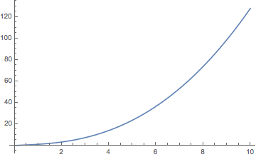
antiD = NDSolveValue[{f'[x] == Sqrt[1 + x^3], f[0] == 0}, f, {x, 0, 10}]

Example usage:

Plot[antiD[x], {x, 0, 10}]

---

Alternatively...

This works because this function can be antidifferentiated (by Mathematica).

antiD = FunctionInterpolation[
 Evaluate @ Integrate[Sqrt[1 + x^3], {x, 0, t}, Assumptions -> 0 < t < 10],
 {t, 0, 10}]

or...

integral[t_?NumericQ] := NIntegrate[Sqrt[1 + x^3], {x, 0, t}];
FunctionInterpolation[integral[t], {t, 0, 10}]

FunctionInterpolation evaluated its argument on a symbolic t. The pattern test ?NumericQ prevents evaluation of NIntegrate until an actual number is substituted for t. See also What are the most common pitfalls awaiting new users?. Note also that this way does many evaluations of NIntegrate, whereas the NDSolve method does just one integration.

Answer 2

There are two aspects in this problem depending on the exact definition of the task, and, as we shall see, both are completely solved by MMA without any additional facility.

The aspects are

a) calculate the interpolation of the definite integral $f=\int_0^t \sqrt{1+x^3} \, dx$

b) calculate the interpolation of the antiderivative $fad=\int\sqrt{1+x^3} \, dx$

Part a) interpolation of Jim's definite integral

There are no problems in interpolating your definite integral if you do it in two steps.

Step 1:

Calculate the definite integral (Mathematica does this exactly)

f = Integrate[Sqrt[1 + x^3], {x, 0, t}, Assumptions -> t >= -1]

(* -> (t^3)^(1/3) Hypergeometric2F1[-(1/2), 1/3, 4/3, -t^3] *)

Step 2:

Do the interpolation

fi = FunctionInterpolation[f, {t, 0, 10}]

(* -> InterpolatingFunction[{{0.`,10.`}},"<>"] *)   

And finally check the equality of f and fi:

Plot[{f, fi[t]}, {t, 0, 10}]

(* skip the picture *)

For completeness:

$Version

(* -> "8.0 for Microsoft Windows (64-bit) (October 7, 2011)" *)

This procedure works fine also with many other functions, e.g. integer powers other than 3 under the sqrt.

Part b) interpolation of the antiderivative

The antiderivative is given by the indefinite integral :

fad = Integrate[Sqrt[1 + x^3], x]

$\frac{2 \left(x+x^4+(-1)^{1/6} 3^{3/4} \sqrt{-(-1)^{1/6} \left((-1)^{2/3}+x\right)} \sqrt{1+(-1)^{1/3} x+(-1)^{2/3} x^2} \text{EllipticF}\left[\text{ArcSin}\left[\frac{\sqrt{-(-1)^{5/6} (1+x)}}{3^{1/4}}\right],(-1)^{1/3}\right]\right)}{5 \sqrt{1+x^3}}$

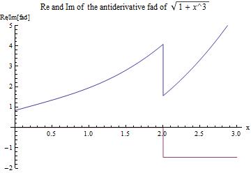
This quantity, besides having a small imaginary part

fad /. x -> 1.25

(* -> 2.34276 - 1.17815*10^-16 I *)

has a dicontinuity in both Re and Im:

Plot[{Re[fad], Im[fad]}, {x, 0, 3}, PlotRange -> {-2, 5}, 
 PlotLabel -> "Re and Im of the antiderivative fad of \!\(\*SqrtBox[\(1 + \
x^3\)]\)", AxesLabel -> {"x", "Re/Im[fad]"}]

Discontinuities of antiderivatives are quite common, and they have been discussed in this community several times (cf. for example Mismatch between numerical and analytic evaluation of an integral)

This could potentially cause a problem for FunctionInterpolate over an interval including the jump.

But it is not the case here !

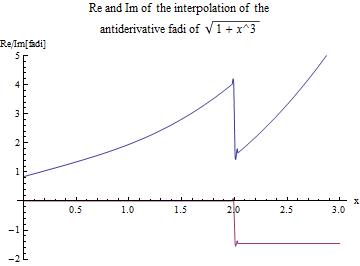
Rather, the interpolation returns the correct complex valued function, with just announcing - as it should do - an accuracy problem connected with the jump:

fadi = FunctionInterpolation[fad, {x, 0, 5}]

FunctionInterpolation::ncvb: FunctionInterpolation failed to meet the prescribed accuracy and precision goals after 6 recursive bisections near x = {1.99219}. Continuing to refine elsewhere. >>

(* InterpolatingFunction[{{0.`,5.`}},"<>"] *)

Visualizing both Re and Im of the interpolation

Plot[{Re[fadi[t]], Im[fadi[t]]}, {t, 0, 3}, PlotRange -> {-2, 5}, PlotLabel -> 
  "Re and Im of the interpolation of the \nantiderivative fadi of \\!\(\*SqrtBox[\(1 + x^3\)]\)", AxesLabel -> {"x", "Re/Im[fadi]"}]

It shows agreement with the original function except, as expected, in the vicinity of the jumps.

Summarizing part b)

the interpolation of the true antiderivative is done perfectly well by Mathematica with only a justified accuracy error message due to the jump.

Conclusion

I have checked the complete code with a fresh kernel and can state that no problems are encountered in version 8 for both interpretations of the problem.

Best regards, Wolfgang