8
$\begingroup$

I want to convert a polynomial in "standard form" to Chebyshev form. Here's one way to do it:

(* My polynomial *) 

pa = Sum[a[i]*t^i, {i, 0, 5}] 

(* "standard form" coefficients of Chebyshev polynomial of same degree *) 

pb = CoefficientList[Sum[b[i]*ChebyshevT[i, t], {i, 0, 5}], t] 

(* helper variable *) 

bs = Table[b[i], {i, 0, 5}] 

Solve[Table[a[i - 1] == pb[[i]], {i, 1, 6}], bs] 

This works, but is there a better (more efficient, more Mathematica-ish) way to do it?

$\endgroup$

5 Answers 5

13
$\begingroup$

Let's say you have a polynomial:

f[x_] := 1 - x + 2 x^2 - 5 x^4
n = 5; (* Polynomial order + 1 *)

Now you have to solve a system of linear equations:

a = Transpose @ PadRight @ Table[CoefficientList[ChebyshevT[k - 1, x], x], {k, n}];
c = LinearSolve[a, CoefficientList[f[x], x]]
(* {1/8, -1, -3/2, 0, -5/8} *)

Sum[c[[k]] ChebyshevT[k - 1, x], {k, n}] // Expand
(* 1 - x + 2 x^2 - 5 x^4 *)

If getting the numerical values of coefficients is sufficient, you can use the discrete Fourier transform, which is an extremely fast method.

$\qquad T_n(x) = \cos(n \arccos x)$

c = 2 MapAt[#/2 &, #, 1]/Sqrt[n] & @ FourierDCT @ f @ Cos[π Range[.5, n]/n]
(* {0.125, -1., -1.5, -9.93014*10^-17, -0.625} *)

Sum[c[[k]] ChebyshevT[k - 1, x], {k, n}] // Expand // Chop
(* 1. - 1. x + 2. x^2 - 5. x^4 *)

P.S. The last method can be used for the Chebyshev expansion of an arbitrary function (there can be a problem with Gibbs oscillations, but that is another story).

$\endgroup$
7
$\begingroup$

The matrix implicitly used for the basis conversion in ybeltukov's answer actually has a nice closed form. You can use this to perform the conversion directly, without having to use LinearSolve[]:

pcmat[n_Integer?NonNegative] := SparseArray[{{j_, k_} /; j <= k && EvenQ[k - j] :> 
      Binomial[k - 1, Quotient[k - 1, 2] - Quotient[j - 1, 2]]/
      2^(k - Boole[j > 1] - 1)}, {n + 1, n + 1}]

Test:

pcmat[4].CoefficientList[1 - x + 2 x^2 - 5 x^4, x]
   {1/8, -1, -3/2, 0, -5/8}

Having the explicit basis change matrix available allows us to study the numerical stability of the conversion. In particular, we can do an analysis similar to the one in this answer, and look at the growth of the condition number of the basis change matrix for various degrees:

Table[Ceiling[Log10[LinearAlgebra`MatrixConditionNumber[pcmat[k]]]], {k, 15}]
   {0, 1, 1, 2, 2, 3, 3, 3, 4, 4, 5, 5, 5, 6, 6}

This says, for instance, that you can lose up to $6$ significant figures when converting a degree-$15$ polynomial in the monomial basis to Chebyshev form.


For completeness, here's the routine for the inverse matrix (for converting from the Chebyshev basis to the monomial basis):

cpmat[n_Integer?NonNegative] := 
      SparseArray[{{1, k_} /; OddQ[k] :> (-1)^Quotient[k, 2],
                   {j_, k_} /; 1 < j <= k :> Cos[(k - j) π/2] 2^(j - 2)
                   Binomial[(k + j)/2 - 2, (k - j)/2] (k - 1)/(j - 1)},
                  {n + 1, n + 1}]
$\endgroup$
6
$\begingroup$

Another possibility is to use Salzer's algorithm (previously used here) to perform the basis conversion:

poly = 1 - x + 2 x^2 - 5 x^4;
c = CoefficientList[poly, x];
n = Length[c] - 1; Remove[a];
a[0, 2] = c[[n - 1]] + c[[n + 1]]/2;
a[1, 2] = c[[n]]; a[2, 2] = c[[n + 1]]/2;
Do[
   a[0, k + 1] = c[[n - k]] + a[1, k]/2;
   a[1, k + 1] = a[0, k] + a[2, k]/2;
   Do[
      a[m, k + 1] = (a[m + 1, k] + a[m - 1, k])/2,
      {m, 2, k - 1}];
   a[k, k + 1] = a[k - 1, k]/2;
   a[k + 1, k + 1] = a[k, k]/2,
   {k, 2, n - 1}];

ccof = Table[a[m, n], {m, 0, n}]
   {1/8, -1, -3/2, 0, -5/8}
$\endgroup$
5
$\begingroup$

This is probably similar to Salzer's algorithm J.M. refers to, but it seemed easier to figure it out from the recurrence relation $$T_{n+1} = 2x\,T_{n} - T_{n-1}$$ From it, we get the following identity for multiplying by $x$: $$\eqalign{ x\, T_0 &= T_1 \cr x\, T_{n} &= \frac{1}{2}\,T_{n+1} - \frac{1}{2}\,T_{n-1}, \quad n \ge 1\cr }$$ From the Horner form $$p(x) = x\, (x\, (x\, (x\, (a_n\, x+a_{n-1})+a_{n-2})+\cdots)+a_1)+a_0$$ we can see that constructing the polynomial can be done by repeated application of the identities above and the relation $a_k = a_k T_0$. It follows that multiplying by $x$ is a linear operation represented by the matrix $$ X=\left( \begin{array}{ccccc} 0 & \frac{1}{2} & & & \\ 1 & 0 & \frac{1}{2} & & \\ & \frac{1}{2} & 0& \ddots & \\ & & \ddots & \ddots & \frac{1}{2} \\ & & & \frac{1}{2} & 0 \\ \end{array} \right) $$

(* n x n Chebyshev multiplication operator:
    chebX[n].cs  multiplies length  n  Chebyshev series  cs  by  x  --
    the series must end in zero or the degree  n-1  term will be lost *)
chebX[n_Integer /; n >= 3] := 
  SparseArray[{{2, 1} -> 1, Band[{3, 2}] -> 1/2, 
    Band[{1, 2}] -> 1/2}, {n, n}];
chebX[2] := SparseArray[{{2, 1} -> 1, Band[{1, 2}] -> 1/2}, {2, 2}];
chebX[1] := SparseArray[{{1, 1} -> 1}, {1, 1}];

J.M.'s example:

poly = 1 - x + 2 x^2 - 5 x^4;
p = Reverse@CoefficientList[poly, x];
n = Length[p];
X = chebX[n];
Fold[X.# + SparseArray[{1 -> #2}, n] &, SparseArray[{}, n], p] // Normal
%.Table[ChebyshevT[n, x], {n, 0, 4}]
% // Expand
(*
  {1/8, -1, -(3/2), 0, -(5/8)}                           -- Coefficients
  1/8 - x - 3/2 (-1 + 2 x^2) - 5/8 (1 - 8 x^2 + 8 x^4)   -- Chebyshev form
  1 - x + 2 x^2 - 5 x^4                                  -- Expanded power series form
*)

Here's a general function:

Clear[chebForm, chebX, chebFunc];

chebFunc[c_?VectorQ, dom_][x_] := chebFunc[c, dom, x];
chebFunc[c_?VectorQ, {a_, b_}, x_?NumericQ] := 
  ChebyshevT[Range[0, Length[c] - 1], (2 x - (a + b))/(b - a)].c;
Normal[chebFunc[c_?VectorQ, {a_, b_}, x_]] ^:= 
  ChebyshevT[Range[0, Length[c] - 1], (2 x - (a + b))/(b - a)].c;

(* Chebyshev multiplication operator (same as above) *)
chebX[n_Integer /; n >= 3] := 
  SparseArray[{{2, 1} -> 1, Band[{3, 2}] -> 1/2, 
    Band[{1, 2}] -> 1/2}, {n, n}];
chebX[2] := SparseArray[{{2, 1} -> 1, Band[{1, 2}] -> 1/2}, {2, 2}];
chebX[1] := SparseArray[{{1, 1} -> 1}, {1, 1}];

(* convert polynomial to Chebyshev series *)
chebForm[poly_, x_] := chebForm[poly, {x, -1, 1}];
chebForm[poly_, {x_, a_, b_}] := Module[{p, n, X},
  p = Reverse@CoefficientList[poly /. x -> (b - a)/2 x + (a + b)/2, x];
  n = Length[p];
  X = chebX[n];
  (* nested multiplication (Horner) *)
  chebFunc[Fold[X.# + SparseArray[{1 -> #2}, n] &, SparseArray[{}, n], p], {a, b}]
  ]

Example: (Normal converts the chebFunc to a Chebyshev series in explicit polynomial form.)

cp = chebForm[poly, x];
cp[x]
% // Normal
% // Expand

Mathematica graphics

The Chebyshev series is particularly (numerically) accurate over the interval $[-1,1]$. One can pass a domain $[a,b]$ that is rescaled to $[-1,1]$:

cp = chebForm[poly, {x, -2, 3}];
cp[x]
% // Normal
% // Expand
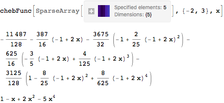
Mathematica graphics

$\endgroup$
0
$\begingroup$

in a more compact, terser way, I would say :
Solve[Thread[Array[a, 6, 0] == pb], Array[b, 6, 0]]
with just the notations Array and Thread thown in.
This avoids explicit (over-)use of Table.

$\endgroup$

Your Answer

By clicking “Post Your Answer”, you agree to our terms of service and acknowledge you have read our privacy policy.